Hubble
Constant
An Expansion Simulator
(built from a prayer and a vision)
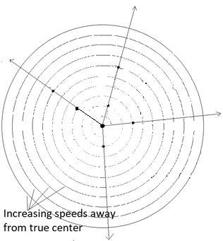
Expansion
motion away from a center, under inertia, could produce observations in our
Universe, including relative acceleration:
To whom it may concern: This is not a scientific paper. I
was reading an article about science building an underground laboratory to
search for Dark Energy and I stopped to pray. I am a Christian and I prayed
saying, “Lord, what is this Dark Energy they’re looking for?” Instantly, I had
a vision. Just as instantly I felt I had seen that space itself was
expanding. I searched the internet for “space itself expanding”, and learned
this is exactly what science believes. With that, I realized that the vision
had shown me what they were looking for. That was enough for me, but that
weekend I ran into a friend who was taking an astronomy class at a local
university. I told him my vision and he said, “The Universe doesn’t have a
center.” Because of the vision, I objected.
Two years later, I heard someone talking about Dark Energy
again on the radio. That brought the vision back into my mind and I designed a
simulator based on the motion I had seen. That motion was all mass expanding
away from a center in the pattern of stretching elastic attached at center. I still
knew little to nothing about observations made in our Universe, only what I
read about the day I googled “space itself expanding, which is what Dr. Hubble
saw.
Below is a list of strange observations coming out of my
simulations. When I googled them, I found they are not so strange. I learned
that modern theory insists space has no center, because it was not possible
that we are at center. My expansion motion had all mass moving away from a
clear center, and was offering another explanation of how it is that every
observer perceives himself at the center of it. I tried to get comments about
my results, but because my expansion pattern offered a clear center, I could
not get anyone to hear me, much less help me. I had to do it myself. Since I
have no math skills, I built a simulator.
Observations
offered by this Simulator:
·
An illusion of center, no matter where the observer is, or when.
·
The actual velocity of every object is away from center. Its
value depends on its distance from center. In fact, it’s simply (velocity
directly away from center) = (Distance from center) / (Age of Expansion).
·
 The relative velocity, with which every object is moving
away from every other, also depends on their distance apart, Relative Velocity
= (distance separated)/(Age of Expansion).
The relative velocity, with which every object is moving
away from every other, also depends on their distance apart, Relative Velocity
= (distance separated)/(Age of Expansion).
·
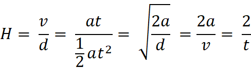
All expansion motions, actual and relative, are related. There
is a relationship factor unique to the moment in time of Expansion by which any
motion can be determined by knowing this factor and how far the object is from
center or its velocity: H = 1/t = v/d.
·
H is easier to calculate by measuring distant objects, the
further the better, because the “noise” in distance measurements is smoothed
out.
·
H is difficult to measure in “local” objects, because they are
just not diverging away from the observer significantly, the closer the more
difficult, and the scope of “local” expands with expansion age.
·
The Hubble Value reduces with each tick of the clock (H = 1/t).
·
With extreme age of Expansion, the Hubble Value will appear to
become a solid constant, good for longer and longer periods of time, depending
on the sensitivity of measurements.
·
If everything is moving away from everything else under this
relationship, and if at the beginning the Universe is homogeneous, then gravity
is naturalized and it will remain homogeneous throughout the history of it, except,
maybe, the outer reaches.
·
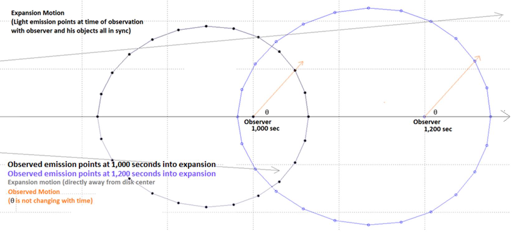
If an observer, and his Center of Momentum, gets out of sync in
this expansion pattern, acceleration shows up in his observed (relative)
expansion motions, when there is none in the actual expansion motion.
·
As gravity clumps mass together, it will pull objects out of sync
in the pattern, but the center of momentum will remain in sync, preserving the
illusions, including that of center for all observers.
·
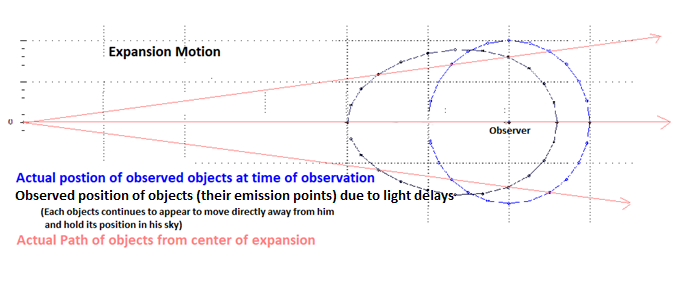
Light delayed viewing will present to the observer a Hubble
Constant Value consistent with the time it is observed, rather than the time the
light was emitted.
·
Gravitational Lensing, producing multiple images of the same light
emission source, will present any observer with the same value of the Hubble
Constant value, no matter how much time is between receipt of the images, or
the path of each to the observer. (This simulator also suggests that lensing
could be used to determine the distance traveled by the light of every path
without knowing the distance of either path of light, if the images are synced.
·
Dark Flow is an observation reported by NASA of the appearance of
strange local motion, or a local expansion within the broader expansion. This
model predicts such a motion and it is an illusion.
·
This simulator might offer a reason CMB and observations offer
two different Hubble Constant values. In fact, it suggests the two would only
be the same if Expansion and the “flash” happened at the same time. It also
offers a relationship between the two values.
The
Vision:
In the vision, I saw a giant hand come in from the right. In
it was a strip of elastic. It attached one end to a surface and then pulled the
other. As it stretched, I perceived, “This is what they are looking for.” It
is the motion I saw in that stretching band that I used to build my simulator.
At first, I felt He had shown me that space itself was expanding, but my
simulator showed me, maybe, but not necessarily. In my simulator, space itself
did not have to be physically expanding to yield the observations listed above.
It could be just mass moving away from a center under inertia, but in this
pattern. I am not a scientist, I knew virtually nothing about Cosmology, and I
was not looking for any specific characteristics in my simulation other than an
illusion of center, which I quickly found. The features listed above just came
out of it. Therefore, I offer my journey through my simulations below, to
whomever is interested. I just want to know, in the end, if the vision was so.
One thing I already know about it, I now understand what they are looking for.
An Expansion
Simulator:
I started out studying what I had seen by placing multiple
dots evenly spaced on an elastic strip and stretching it from one end. I could
see an illusion of center for every observer placed at any point along its
length as it is stretched. I could also see that the density of the objects
dropped evenly as the strip was stretched. I could also see that each object’s
velocity depended on its distance from the attached end, and that, even though
any observer would see all objects moving away from him, all objects were
always moving directly away from the attached end.
I then wanted to know if the same would be true within a
stretching sphere. I imagined a sphere and determined that if I could show
this is true with a thin disk cut from it, then it would be true for the whole
sphere. The sliver would have to include the center of the sphere, the
observer and an object being observed.
To simulate expansion of my thin disk, I imagined thousands
of elastic strips attached at its center, with objects and observers attached
anywhere on them. I then stretched (expanded) the disk by pulling each strip simultaneously
away from center, all at the same steady rate. When I stretched the disk, strange
observations emerged from my simulations, but when I googled them, I learned
they are actually being observed.
Each object moved with the stretching band it was attached
to (its axis is its path away from center). In the charts below, I stretched each
axis for a set time before pausing to evaluate how each object was moving. At
each pause (steady rate or accelerating), the new position of each object could
be determined in various ways. (On the day I read about the Hubble Motion
formula, I applied it to my charts and saw how it worked and added it, but by
then, I had already seen in a disk what Dr. Hubble had seen in space.)
If the stretching was a steady rate, all objects had a
steady velocity, moving away from center, and each object’s speed depended on
its distance from center, the value increasing with distance. Each pause had
its own Hubble Value that could be used to show a relationship of all actual
motion away from center. The same Hubble Value showed the same relationship
between all relative motion between any two objects. It was Hubble Motion within
Hubble Motion, just like with the stretching band. This is what Dr. Hubble
might have witnessed.
I determined the change of position of each object at each
pause (steady rate or accelerating) by multiplying the new length of the axis
(new radius of the disk at each pause) by the ratio of the object’s starting
distance from center divided by the starting length of the band (original radius
of disk).
New position of object = (initial distance of
object from center / initial length of axis) * (rate of expansion * age of
expansion)
If this expansion is an acceleration;
New position of object = (initial distance of object
from center / initial length of axis) * (.5 * acceleration rate * age of
expansion^2)
It turned out that the position of each object could have
been determined through time once the velocity of each object is known, using d
= v * Age of Expansion. This model assumes everything started out at center,
which meant that for my model, H = v/d = 1/Age of Expansion.
The Simulations:
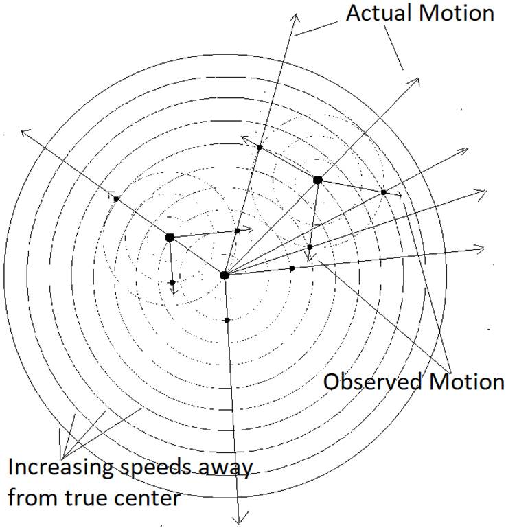
I randomly placed an observer within my disk and drew an
axis that passed through him and the center of the disk (see image below). I
started out assuming no gravity and no delays of observation due to light
propagation. I drew a “circle of observation” of a random radius around my
observer. I placed objects on this circle for him to watch and to collect data as
the disk expanded (data charts below). As I placed each object on his circle, I
calculated the angle at disk center between the observer and his objects and
the distance of the object from center. Just like with my observer, I drew an
axis from center through each object that I could “stretch” and give it motion
due only to expansion.
I expanded my tiny sphere by “pulling” each axis at the same
rate simultaneously, pulling each outward from center. The resulting motion of each
object was solely due to expansion determined by its position on each
stretching axis. Each axis represented the actual path of each object’s motion.
For my first simulation, I pulled each axis at a steady rate, all expansion
motion was therefore away from center at steady velocities. I later ran
simulations pulling at accelerated rates. In both forms of expansion, the
Hubble Law remained valid throughout, and all observations present within this
pattern of motion were preserved. All actual motion was away from center, and
the illusions of center were present in all relative motions.
My initial goal was to examine how this movement affects my observer’s
perspective of each object on his observation circle(s). Later, I added the
delays of observation due to the speed of light and the effects of gravity.
My analysis suggests that this pattern of motion could
explain what Dr. Hubble observed. He was looking into an illusion of center. He
was indeed seeing from the perspective of center, as if at center, yet not.
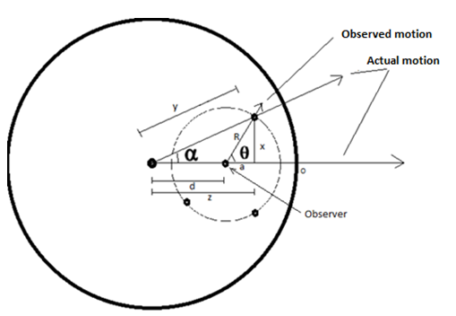
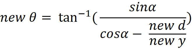
Expansion motion, and a “Circle of Observation”:
|
R= Radius of
circle around Observer
|
y=distance
from center of disk to object being observed
|
θ =
angle from Observer’s axis to the Object being observed
|
|
x = opposite
side of Observer’s view of object
|
d=distance
from center of disk to Observer
|
α = Angle at center of disk between
object and Observer
|
|
a= adjacent
side of Observer’s view of object
|
z = distance
from center of disk to x
|
O = radius of
disk
|
Steady Rate Expansion:
The idea here is that all mass began compacted at center,
but my first pause to examine the expansion began at 15 seconds into the
expansion process. I stretched the disk at a steady 10cm/sec (disk radius
change rate). I randomly placed my Observer (“Y”) at 75cm from disk center and
created three “Circles of Observation” around him. One of radius 50cm, one at
60, and another at 55.73. I placed objects on each circle by randomly
selecting angles in his sky where he can see them. (The angle is between his
axis and the objects.) As the “stretching” progressed, I could track where
those objects are in his sky, how that angle changes.
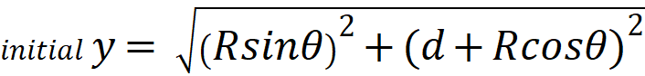
Locate the position of y (distance from center) for all
objects placed on the Observer’s “Circles of Observation” based on Observer Y’s
distance from center (75cm). Radius R of each circle is selected at random, as
well as positions in degrees (θ) in the observer’s sky for each object.
Distance of objects from center
of disk
|
Time into expansion
|
Hubble
Value
|
Radius of Disk
after each expansion
(Initial O)
|
Observer Y
(Initial d)
|
Object A
R = 50
θ=60 deg
(Initial y)
|
Object B
R = 50
θ=200 deg
(Initial y)
|
Object C
R = 60
θ=60 deg
(Initial y)
|
Object D
R = 60
θ=200 deg
(Initial y)
|
Object E
R = 55.73
θ=51.1 deg
(Initial y)
|
|
15 sec
|
0.066667
|
150cm
|
75cm
|
108.97
|
32.82
|
117.15
|
27.71
|
118.24
|
What is the angle at center of the disk between the observer
and the object being observed?
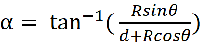
Angle from center between
observer and each object
|
Time into expansion
|
Radius of Disk
after each expansion
(Initial O)
|
Observer Y
|
Object A
R = 50
θ=60 deg
α
|
Object B
R = 50
θ=200 deg
α
|
Object C
R = 60
θ=60 deg
α
|
Object D
R = 60
θ=200 deg
α
|
Object E
R = 55.73
θ=51.1 deg
α
|
|
15 sec
|
150cm
|
---
|
23.41
|
-31.40
|
26.33
|
-47.78
|
21.52
|
Then stretch the disk by “pulling” each axis at a set rate
for a set amount of time. I paused the stretch to calculate how each object moved
along its own axis. This will be the motion of objects along their axis due
only to this expansion pattern.

Actual Motion away from center
of each object along its own axis as expansion progresses
|
Time into expansion
|
Hubble
Value
1/Time
|
Radius of Disk
after each expansion
(new O)
|
Observer Y
(new d)
|
Object A
R = 50
θ=60 deg
(new y)
|
Object B
R = 50
θ=200 deg
(new y)
|
Object C
R = 60
θ=60 deg
(new y)
|
Object D
R = 60
θ=200 deg
(new y)
|
Object E
R = 55.73
θ=51.1 deg
(new y)
|
|
16 sec
|
0.062500
|
160 cm
|
80.00
|
116.24
|
35.01
|
124.96
|
29.56
|
126.12
|
|
50 sec
|
0.020000
|
500cm
|
250.00
|
363.23
|
109.40
|
390.50
|
92.37
|
394.13
|
|
51 sec
|
0.019608
|
510cm
|
255.00
|
370.50
|
111.59
|
398.31
|
94.21
|
402.02
|
|
5000 sec
|
0.000200
|
50,000cm
|
25,000.00
|
36,323.33
|
10,940.00
|
39,050.00
|
9,237.50
|
39,413.33
|
|
5001 sec
|
0.000200
|
50,010cm
|
25,005.00
|
36,330.60
|
10,942.19
|
39,057.81
|
9,239.35
|
39,421.22
|
|
Actual velocity due to expansion motion
|
---
|
5cm/sec
|
7.27cm/sec
|
2.18cm/sec
|
7.81cm/sec
|
1.85cm/sec
|
7.89cm/sec
|
Calculations of position came from the motion generated as
each axis is being stretched like elastic pinned at center, but the resulting
motions are a steady velocity.
Therefore, this motion could be a simple drifting away from a
center under inertia.
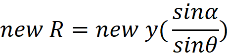
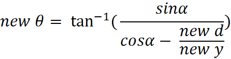
For each movement, strictly by the expansion process, re-calculate
the new angle θ of each object with respect to the observer, where will he
now have to look to find that object in his sky?
Observed Position: Effect of
expansion motion on the position of each object in our observer’s sky
|
Time
|
Object A
R = 50, θ=60 deg
new θ
|
Object B
R = 50, θ=200 deg
new θ
|
Object C
R = 60, θ=60 deg
new θ
|
Object D
R = 60, θ=200 deg
new θ
|
Object E
R = 60, θ=60 deg
new θ
|
|
15 sec
|
60
|
200
|
60
|
200
|
51.1
|
|
16 sec
|
60
|
200
|
60
|
200
|
51.1
|
|
50 sec
|
60
|
200
|
60
|
200
|
51.1
|
|
51 sec
|
60
|
200
|
60
|
200
|
51.1
|
|
5000 sec
|
60
|
200
|
60
|
200
|
51.1
|
|
5001 sec
|
60
|
200
|
60
|
200
|
51.1
|
|
Change of position in observer’s sky
|
unchanged
|
unchanged
|
unchanged
|
unchanged
|
Unchanged
|
At each pause, how has the radius of each “circle of
observation” been affected? This is measured by the relative motion of each
object to the observer, the actual distance between them.
Relative (Observed) Motion: Distance
measured by observer to each object
|
Time
|
Hubble
Value
|
Object A
R = 50, θ=60 deg
new R
|
Object B
R = 50, θ=200 deg
new R
|
Object C
R = 60, θ=60 deg
new R
|
Object D
R = 60, θ=200 deg
new R
|
Object E
R = 55.73, θ=51.1 deg
new R
|
|
15 sec
|
0.066667
|
50.00
|
50.00
|
60.00
|
60.00
|
55.73
|
|
16 sec
|
0.062500
|
53.33
|
53.33
|
64.00
|
64.01
|
59.45
|
|
50 sec
|
0.020000
|
166.67
|
166.67
|
200.00
|
200.00
|
185.77
|
|
51 sec
|
0.019608
|
170.00
|
170.00
|
204.00
|
204.00
|
189.48
|
|
5000 sec
|
0.000200
|
16,664.78
|
16,667.07
|
19,999.15
|
19,999.04
|
18,577.41
|
|
5001 sec
|
0.000200
|
16,668.12
|
16,670.40
|
20,003.14
|
20,003.03
|
18,581.13
|
|
Relative velocity due to expansion
|
|
3.33 cm/sec
|
3.33 cm/sec
|
4.00 cm/sec
|
4.00 cm/sec
|
3.72 cm/sec
|
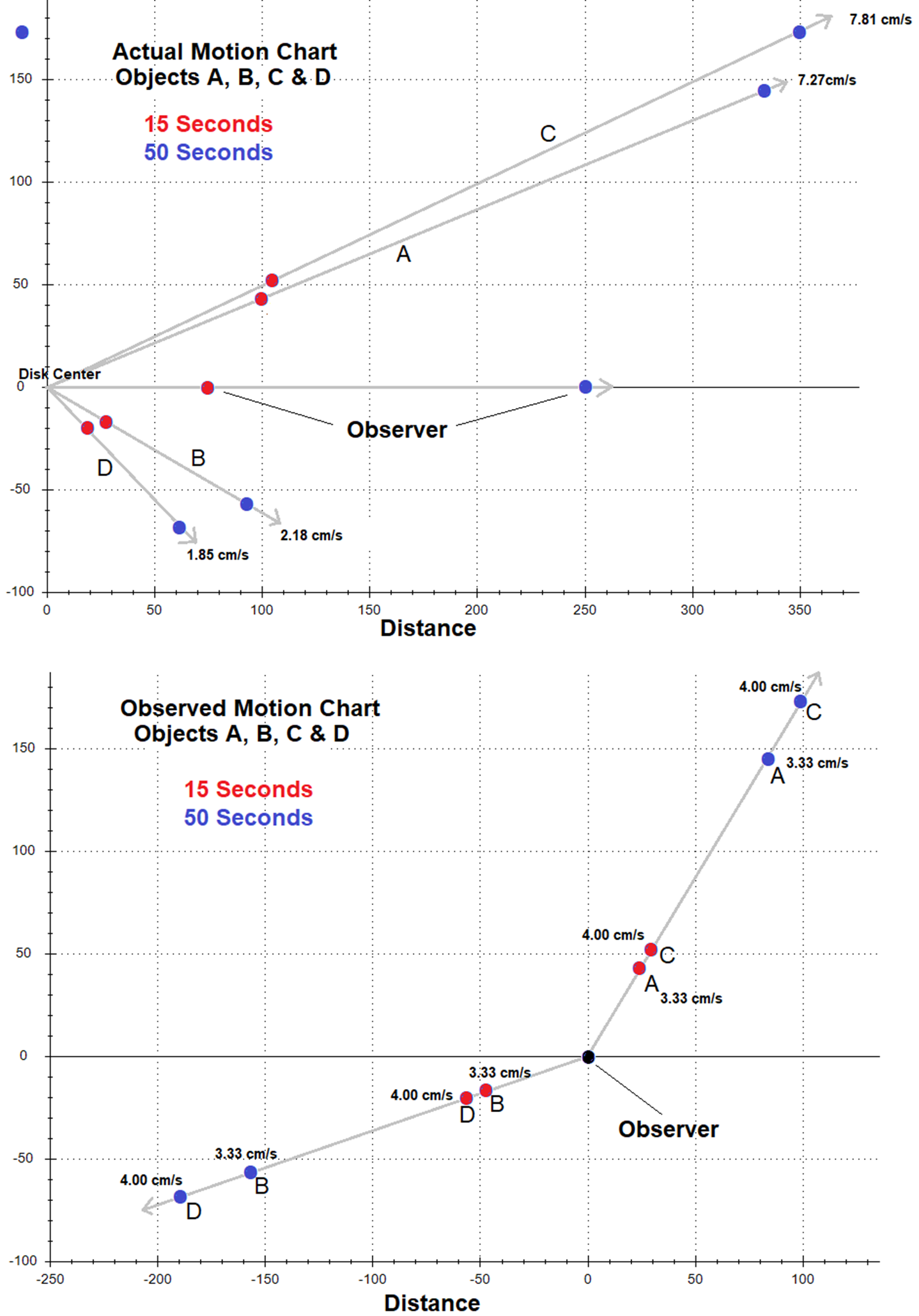
Analysis:
All motion was due to pulling every axis at a steady rate. Each
object’s motion was directly away from center. The resulting calculations show
that this motion kept each object on the observer’s original circle of
observation in the exact position where he first saw it. This expansion motion
accomplished this while simultaneously increasing the radius of each circle,
moving every object on the circle away from the observer. Each pause could be
evaluated using the Hubble formula. This motion created an illusion that the
observer was standing at the center of an expansion process, every object
receding from him in all directions. Each object was moving away from center
at a constant velocity, proportional to distance from center. Each object was moving
away from every observer at a constant relative velocity, also proportional to
distance. Every object was moving away from center at a divergent angle (α)
to every other. Every observer would record a redshift when viewing every
other object.
The “Observed Motion” chart turns out to be identical if I
place my observer at different locations with the same configuration for the
same time span of expansion, but his “Actual Motion” chart will change with
position. He cannot tell from his observations that he is in a different place.
Since this includes him standing on true center this pattern of motion presents
every observer with a view of expansion as if he were standing at true center.
He is seeing center, yet not, it is an illusion of center for every observer.
If we place another observer at dead center with the same
configuration of objects his “Observed Motion” chart would be identical to his
“Actual Motion” chart. His “Observed” chart would be identical to Observer Y’s
“Observed” Chart, if data is collected at the same moment of expansion. When
an observer is standing on true center, his “observed” motion is the “actual”
motion. Every other observer is observing relative motions and cannot discern
the actual, either his own or the objects he is observing. He thinks he is at
the center of an expansion.
At each pause, the Hubble value calculated is the same by
all observers. An observer standing at true center watching Observer Y at 50
seconds into expansion would calculate a Hubble value of v/d = 5cm/sec / 250cm
= .02/sec. Observer Y, at the same moment, watching Object A (“Observed Motion”)
would calculate his H as 3.33/166.67 = .02/sec.
Each observer is caught up in their own relationship of
relative motions. Each observer’s relative motions mimic what is observed at
center. This tiny model could therefore be another explanation of why Dr.
Hubble saw an appearance of center.
When I started my simulations all I knew about Cosmology was
Dr. Hubble seeing everything receding. I was unaware of the Hubble formula.
When my data charts resembled what Dr Hubble saw I began to read more about
him. That is when I learned about the Hubble formula. I began to divide
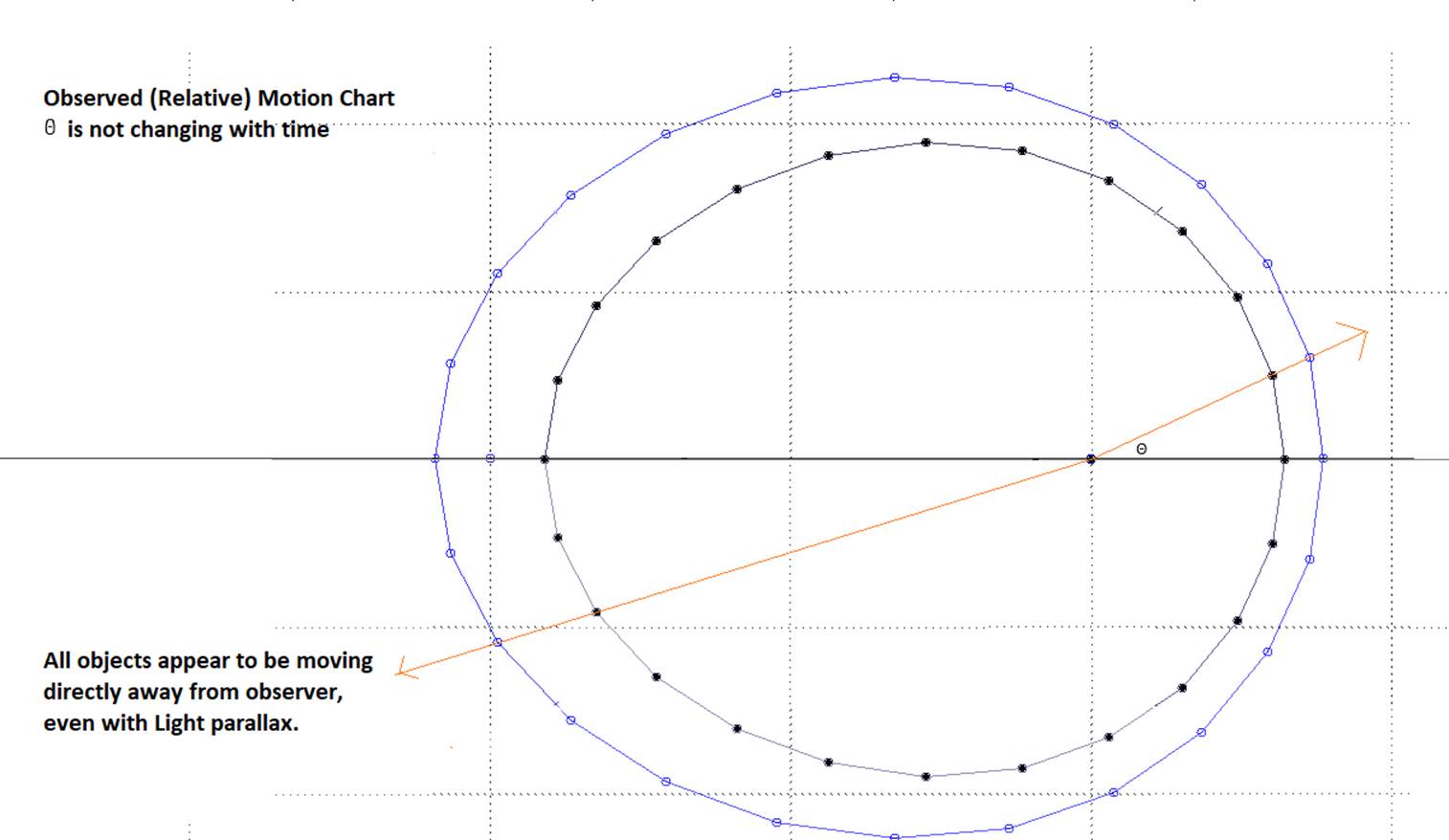
separations between objects in my chart and saw that it nicely describes the
relationships between the observer and all his objects at each pause (row).
For each pause, it could be used to calculate any position from a known velocity
or a velocity from a known position. In time, I saw that in my charts H = 1/t,
where t is the age of the expansion at the time of the pause. I just needed to
know the time of the pause to know H, or I could calculate it from H = vy /
(new y) = vR / (new R). I could see that the Hubble formula was
really just d = vt and this formula could be used to replace my elastic
stretching formula, but I didn’t do that. For example, in my “Actual Motion”
chart, once I knew Observer Y was moving along at 5cm/s, I could have
determined his distance from center by (new O) = 5cm/51sec = 255cm. The Hubble
formula is better for expansion, because it expresses d=vt as a relationship
between all the objects caught up in the expansion process.
“Locally”
Observed Expansion Motion slowing with time:
As I ran more simulations, I could see that close-range
relative motion was slowing with Expansion age. I setup two new simulations to
examine “local” vs “distant” observations of Expansion Motion.
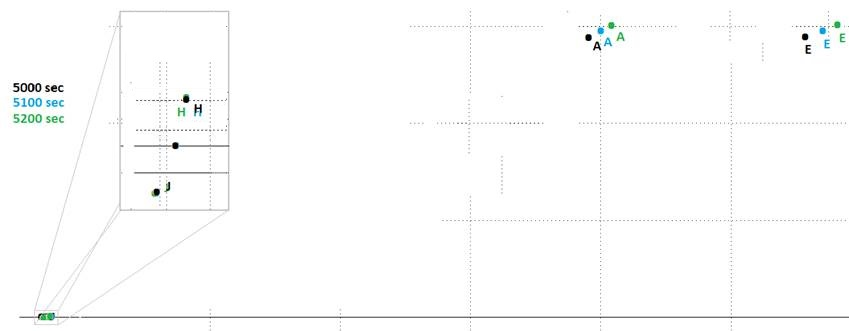
In my first simulation of local Expansion Motion, Observer Y
is still watching Objects A and E, but now the expansion has aged to 5,000
seconds. At 5,000 seconds, Observer Y will have moved to 25,000cm away from
center. I added two new objects in his sky, H and J. These two new objects are
starting out on his original “Circle of Observation” of R=50cm, to represent
“local” observation of Expansion. Objects A and E will represent “distant”
observation of Expansion Motion. They will have move away from Observer Y to
16,664cm and 18,577cm, respectively, and away from center of disk to 36,323cm
and 39,413cm, respectively.
For my second simulation of local relative motion, I placed
a new observer Z at the same 5,000 seconds mark. He is on Observer Y’s axis,
and at Y’s original vantage point of 75cm from center. I added Objects F and G on
a Circle of Observation for him to watch at the same perspective that Y had for
his A and B (starting at the same R and θ).
I let Observer Z see the motion of objects A and E.
Actual Motion: Observer Y and
his objects starting at 5,000 seconds into expansion
|
|
New
Local Objects
|
Original
Non-Local Objects
|
|
Time into expansion
|
Hubble
Value
|
Radius of Disk
after each expansion
|
Observer Y
new d
|
Object H
R = 50
θ=60 deg
new y
|
Object J
R = 50
θ=200 deg
new y
|
Object A
R = 16,664
θ=60 deg
new y
|
Object E
R = 18,577
θ=51.1 deg
new y
|
|
α
|
|
|
|
0.10
|
-0.04
|
23.41
|
21.52
|
|
5000 sec
|
0.000200
|
50,000cm
|
25,000.00
|
25,025.04
|
24,953.02
|
36,323.33
|
39,413.33
|
|
5001 sec
|
0.000200
|
50,010cm
|
25,005.00
|
25,030.04
|
24,958.01
|
36,330.59
|
39,421.21
|
|
5002 sec
|
0.000200
|
50,020 cm
|
25,010.00
|
25,035.05
|
24,963.00
|
36,337.86
|
39,429.09
|
|
5100 sec
|
0.000196
|
51,000 cm
|
25,500.00
|
25,525.54
|
25,452.08
|
37,049.80
|
40,201.60
|
|
5200 sec
|
0.000192
|
52,000 cm
|
26,000.00
|
26,026.04
|
25,951.14
|
37,776.26
|
40,989.86
|
|
Actual velocity due to expansion
|
|
5.00 cm/sec
|
5.01 cm/sec
|
4.99 cm/sec
|
7.26 cm/sec
|
7.88 cm/sec
|
At 5,000 seconds into expansion objects
50cm away from the observer now had virtually the same speed as the observer (divergent
angle α is very small between them). This contrasts with objects at the
same distance from him when expansion was just 10 seconds old.
Observed Motion: Distance measured
by Observer Y to each object
|
|
Local Objects
|
Non-Local Objects
|
|
Time
|
Hubble
Value
|
Object H
R = 50
θ=60 deg
new R
|
Object J
R = 50
θ=200 deg
new R
|
Object A
R = 16,664
θ=60 deg
new R
|
Object E
R = 18,577
θ=51.1 deg
new R
|
|
5000 sec
|
0.000200
|
50.00
|
49.94
|
16,664.12
|
18,577.52
|
|
5001 sec
|
0.000200
|
50.01
|
49.95
|
16,667.45
|
18,581.24
|
|
5002 sec
|
0.000200
|
50.02
|
49.96
|
16,670.79
|
18,584.96
|
|
5100 sec
|
0.000196
|
51.00
|
50.93
|
16,997.40
|
18,949.08
|
|
5200 sec
|
0.000192
|
52.00
|
51.93
|
17,330.68
|
19,320.63
|
|
Relative velocity due to expansion
|
0.01 cm/sec
|
0.01 cm/sec
|
3.33 cm/sec
|
3.72 cm/sec
|
“Local”
(grey box) verses Distant Actual Expansion Motion
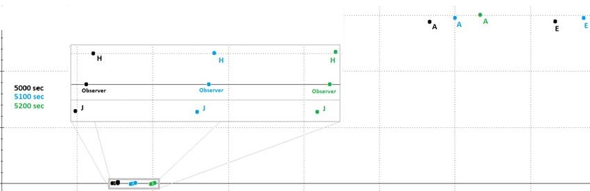
“Local” (grey
box) verses Distant Observed (Relative) Expansion Motion
At 15 seconds into Expansion, Observer Y was 50cm from
Object A and moving away at an expansion motion of 3.33cm/s. Observer Y could
easily measure their relative velocity. When the Expansion aged to 5,000
seconds, A had moved to 36,363cm away, but still moving directly away at an
expansion motion of 3.33cm/s. Observer Y could still easily measure the
relative velocity. However, 5,000 seconds I added the new object H at 50cm
away from Y. Y then measured an expansion motion for H of 0.01cm/s. At 15
seconds into Expansion, object H would have been 75.01cm from center and just
0.15cm away from the Observer. At 15 seconds into expansion, this example of
"local" Expansion Motion was about 0.2cm, but expanded to 50cm at
4,985 seconds later.
For my simulation of Observer Z, I calculated his
perspective of A and E (distance and θ); where are they in his sky?
Actual Motion: Observer Z and
his objects starting at 5,000 seconds into expansion
|
|
Local Objects
|
Non-Local Objects
|
|
Time into expansion
|
Hubble
Value
|
Radius of Disk
after each expansion
|
Observer Z
new d
|
Object F
R = 50
θ=60 deg
new y
|
Object G
R = 50
θ=200 deg
new y
|
Object A
R = 36,254
θ=23.46 deg
new y
|
Object E
R = 39,344
θ= 21.56 deg
new y
|
|
α
|
|
---
|
---
|
23.41
|
-31.40
|
23.41
|
21.52
|
|
5,000 sec
|
0.000200
|
50,000cm
|
75.00
|
108.97
|
32.82
|
36,323.33
|
39,413.33
|
|
5,001 sec
|
0.000200
|
50,010cm
|
75.02
|
109.00
|
32.83
|
36,330.59
|
39,421.21
|
|
5,002sec
|
0.000200
|
50,020cm
|
75.03
|
109.02
|
32.83
|
36,337.86
|
39,429.09
|
|
5,100 sec
|
0.000196
|
51,000cm
|
76.50
|
111.15
|
33.48
|
37,049.80
|
40,201.60
|
|
5,200 sec
|
0.000192
|
52,000cm
|
78.00
|
113.33
|
34.13
|
37,776.26
|
40,989.86
|
|
Actual velocity due to expansion
|
---
|
.02 cm/sec
|
.02 cm/sec
|
.01 cm/sec
|
7.26 cm/sec
|
7.88 cm/sec
|
Observed Motion: Distance measured
by Observer Z to each object
|
|
Local Objects
|
Non-Local Objects
|
|
Time
|
Hubble
Value
|
Object F
R = 50
θ=60 deg
new R
|
Object G
R = 50
θ=200 deg
new R
|
Object A
R = 36,254.52
θ=23.46 deg
new R
|
Object E
R = 39,343.68
Θ=21.56 deg
new R
|
|
5000 sec
|
0.000200
|
50.00
|
50.00
|
36,254.52
|
39,343.68
|
|
5001 sec
|
0.000200
|
50.01
|
50.01
|
36,257.53
|
39,351.55
|
|
5002 sec
|
0.000200
|
50.01
|
50.01
|
36,264.78
|
39,359.42
|
|
5100 sec
|
0.000196
|
50.99
|
51.00
|
36,975.28
|
40,130.68
|
|
5200 sec
|
0.000192
|
51.99
|
51.99
|
37,700.28
|
40,918.68
|
|
Relative velocity due to expansion
|
.01 cm/sec
|
.01 cm/sec
|
7.25 cm/sec
|
7.87cm/sec
|
The charts suggest that the reason observation of local
expansion in our Universe is so difficult is because as time passes objects moving
with significant relative Expansion Motion have moved out of our local space. As
Expansion progresses, more and more of the objects close to us are barely
showing any relative Expansion Motion, although it is there. Those objects have
always been moving with very slow relative Expansion Motion. From the
beginning, these are objects that are moving at virtually the same speed away
from center and at very small angles of divergence (α).
Therefore, relative (observed) Expansion Motion of close
objects will fall toward insignificance as expansion grows old. The data charts
suggest that distances from an observer considered “local” in scope (Expansion
Motion difficult to observe) grows larger and larger as expansion ages.
The Pattern
as an Accelerating Expansion – pulling each axis at an accelerated rate
If Expansion Motion is an acceleration can simulate it by
pulling each axis at an accelerated rate, but unlike steady rate expansion this
could not be inertia.
Instead of objects moving away from center at constant velocities
at values that increase with distance from center, now objects are moving with
constant accelerations at values that increase with distance from center. At
each pause, there is still a Hubble Formula relationship between all objects
caught up in the expansion, H = v/d, but now H = 2/(Age of Expansion).
If looking at a single pause in the simulation you cannot
tell whether the motion is steady rate or accelerating, except the H value. All
observer’s still record all objects receding directly away, but now relative
motion is an acceleration.
If Expansion Motion slows and speeds up this simulation can
do either and still present observations of center, homogeneous expansion, and
insignificant local relative motion.
Object A: Actual Motion with a
forced acceleration of each object along its own axis away from center (without
viewing delays of light propagation)
|
Time into expansion
|
Hubble
Value
2/Time
|
Observer Y
new d
|
Observer Y
Velocity
(d)
|
Object A
R = 50
θ=60 deg
(y)
|
Object A
Velocity
|
Object A
Observed
Distance
|
Object A
Observed
Velocity
|
Object A
θ
|
|
15 sec
|
0.13333
|
75.00
|
10.00
|
108.97
|
14.53
|
49.99
|
6.67
|
60
|
|
16 sec
|
0.125
|
85.33
|
10.67
|
123.98
|
15.50
|
56.88
|
7.11
|
60
|
|
50 sec
|
0.04
|
833.33
|
33.33
|
1,210.78
|
48.43
|
555.49
|
22.22
|
60
|
|
51 sec
|
0.03922
|
867.00
|
34.00
|
1,259.69
|
49.40
|
577.93
|
22.66
|
60
|
|
5000 sec
|
0.0004
|
8,333,333.33
|
3,333.33
|
12,107,777.78
|
4,843.11
|
5,554,928.73
|
2,221.97
|
60
|
|
5001 sec
|
0.0004
|
8,336,667.00
|
3,334.00
|
12,112,621.37
|
4,844.08
|
5,557,150.92
|
2,222.42
|
60
|
|
Acceleration due to expansion
|
|
0.67cm/s/s
|
|
0.97cm/s/s
|
|
0.44cm/s/s
|
|
Object B: Actual Motion with a
forced acceleration of each object along its own axis away from center (without
viewing delays of light propagation)
|
Time into expansion
|
Hubble
Value
2/Time
|
Observer Y
(d)
|
Observer Y
Velocity
|
Object B
R = 50
θ=200 deg
(y)
|
Object B
Velocity
|
Object B
Observed
Distance
|
Object B
Observed
Velocity
|
Object B
θ
|
|
15 sec
|
0.13333
|
75.00
|
10.00
|
32.82
|
4.38
|
50.00
|
6.67
|
200
|
|
16 sec
|
0.125
|
85.33
|
10.67
|
37.34
|
4.67
|
56.89
|
7.11
|
200
|
|
50 sec
|
0.04
|
833.33
|
33.33
|
364.67
|
14.59
|
555.57
|
22.22
|
200
|
|
51 sec
|
0.03922
|
867.00
|
34.00
|
379.4
|
14.88
|
578.01
|
22.67
|
200
|
|
5000 sec
|
0.0004
|
8,333,333.33
|
3,333.33
|
3,646,666.67
|
1,458.67
|
5,555,690.92
|
2,222.28
|
200
|
|
5001 sec
|
0.0004
|
8,336,667.00
|
3,334.00
|
3,648,125.48
|
1,458.96
|
5,557,913.41
|
2,222.72
|
200
|
|
Acceleration due to expansion
|
|
0.67cm/s/s
|
|
0.29cm/s/s
|
|
0.44cm/s/s
|
|
The Source
of the Illusion of Center
The source of the illusion of center, all objects
receding directly away at the same rate per distance in all directions of the
observer’s sky, is in the observer’s inability to perceive his own motion due
to expansion. The illusion is in the interaction of vector motions within this
pattern.
Object’s Expansion velocity vectors as viewed by observer:
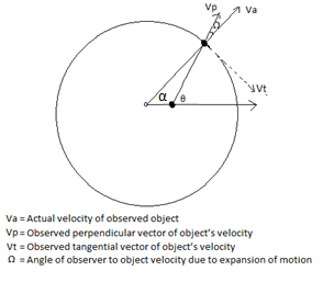
Ω
= θ – α
(θ = angle of the object on the viewing
circle)
Vp = Va cos(Ω)
Vt = Va sin(Ω)
Observer’s Expansion Velocity vectors as projected onto the
observed object:
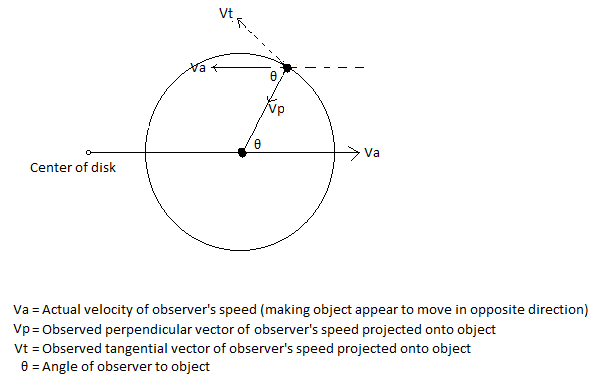
θ = observer’s angle to object
Vp
= - Va cos(θ)
Vt
= - Va sin(θ)
Using data from the original chart above, Observer Y was
watching Object A when it was 50cm away and 60 degrees from his expansion
motion. He determined that it was moving directly away from him at 3.33cm/sec.
He found that every object 50cm away was moving directly away from him at the
same speed.
The actual Expansion velocity of Object A was 7.27cm/sec
directly away from disk center, and the divergent angle between the observer
and Y at true center was 23.41 degrees.
Vectors of Observer Y’s Expansion
motion projected onto Object A:
Ω = 60 - 23.41 = 36.59
degrees
Va =
7.27 cm/sec
Vp =
7.27cm/sec * cos(36.59) = 5.84 cm/sec
Vt =
7.27 cm/sec * sin(36.59) = 4.33 cm/sec
Object A’s Expansion motion as
viewed by Observer Y:
Va = - 5.00
cm/sec (from data chart)
Vp = - 5.00 cm/sec
* cos(60) = - 2.50 cm/sec
Vt = - 5.00
cm/sec * sin(60) = - 4.33 cm/sec
For this expansion pattern all movement is part of the
Hubble relationships (v=Hd):


Observer Y’s relative Expansion velocity (measured perpendicular
motion) for object A is the sum of their two “actual motion” perpendicular vectors;
Observed Velocity = 5.84 – 2.50 =
3.34 cm/sec.
Observer Y’s tangential Expansion velocity is the sum of their
two tangential vectors:
Tangential Motion in the observer’s
sky = 4.33 – 4.33 = 0.
This relationship is true between all objects moving away
from center in this Expansion pattern. In this pattern of motion, our observer
cannot see the tangential vector of Expansion Motion, because his own is
exactly masking the object’s to nil.
The result is that each object on each circle is viewed as
moving the same speed directly away from him, when in fact they are neither
moving directly away, nor the same speeds, unless the observer happens to be
special, standing on dead-center of the disk. Center is an illusion.
The Hubble Constant
The Hubble Constant is defined as H = v / d. In this model,
v is the observed or actual velocity, and d is the distance from observer or
from center, respectively. Here, H is not a constant but a value good for
“moments” in time. As the expansion ages, H does become more of a constant. At
any moment in time an H can be measured anywhere in the disk, and then be used for
the whole within that moment, but its value changes as expansion advances. Dr.
Hubble would have been measuring “observed” motion within the illusion, a
product of relative motion, and his measurement of H would be accurate for the
“actual”, which he could not discern.
Using “Actual” motion of Object A, at the 15 second mark, yields
H = 7.27/108.97 = .067. Using the “Observed” motion at the same moment,
Observer Y would calculate H = 3.33/50 = .067. If Dr. Hubble was looking out
into this universe, he was not able to see the actual motion, yet his data gave
him the actual H of expansion for that moment.
I designed my data such that Object A and Object E start out
at 10cm apart at the 15 second moment in expansion. If H at 15 seconds is .067,
then the two objects should be expanding away from each other at v = H * d = .67cm/sec.
To check that, I calculated the actual distance between the two objects due to expansion
motion at the 16 second mark. The separation grew to 10.67cm, which is a
velocity of .67 cm/sec. The two results agree.
As expansion gets older, the H value becomes increasingly
stable. At the 5,000 seconds mark the H value dropped to .002. It stayed that
value for a long period of time (at 3 significant digits). In the second data chart
when the expansion age was even more advanced, H dropped to 0.00026. At this
more advanced stage, even using 5 significant digits, the H value did not
register change over 200 seconds. Calculated values for H would be more and
more of an estimate as the universe ages.
Hubble Value of this expansion model:
H = Actual velocity of any object
away from center / distance from center
OR
H= Observed velocity/observer’s
distance to object
OR
H = Observed net velocity between
two objects / separation between them
OR
If H = v / d, (for pure
expansion motion that is not an acceleration)
v = (distance between any two
objects) / (Age of the Universe)
(Any position can count as an
object, even if there is nothing there)
d = (distance between same two
objects)
then,
H = 1 / (Age of the Universe).
If expansion is an acceleration:
For steady rate expansion, the Hubble value for an expanding
disk is the reciprocal of the age of the expansion process. H is therefore independent
of the rate of expansion. If I stretch my disk at 10cm/sec it will have the
same Hubble value at any given time as a disk being stretched at 500cm/sec. An object
that is at 75cm from center 15 seconds into the expansion of a disk being
stretched at 10cm/sec will be at 3,750cm if the same disk is being stretch for
15 seconds at 500cm/sec.
The current Hubble Value reported for our Universe, derived
from observations:
H (derived from observation) =  =
= 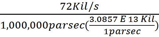 = 2.33 E -18 /s
If this is so, and H is changing with time, then at the
current age of our Universe it would take 58.6M years to observe H changing.
 -
-  = 1 / (2.32E-18/sec) – 1
/(2.33E-18/sec) = 1,849,933,402,397,513sec = 58.6M years
= 1 / (2.32E-18/sec) – 1
/(2.33E-18/sec) = 1,849,933,402,397,513sec = 58.6M years
At 4 significant digits, 1 / (2.332E-18/sec) – 1
/(2.333E-18/sec) = 183,804,743,485,776sec = 5.8M years
At 5 significant digits, 1 / (2.3332E-18/sec) – 1
/(2.3333E-18/sec) = 18,368,658,970,850sec = 582K years
At 6 significant digits, 1 /
(2.33332E-18/sec) – 1 /(2.33333E-18/sec) = 1,836,747,813,490sec= 58K years
At advanced age of the expansion, to
the observer H will appear to be a constant.
The Speed of Light: Hubble Motion and illusions of
center preserved
The calculated data in my original charts
assumed no gravity and no speed of light parallax. The illusions of this
pattern are true instantaneously, but astronomers view objects from great
distances, seeing light emitted from their past. I felt surely that this delay
of our Universe would reap havoc on the illusions seen in this model. Instead,
not only does it maintain Hubble motion and the illusions of center, but it
adds a new illusion. In steady rate expansion the delay somehow converts the
Hubble value at the time the light was emitted, in the past, to the value at the
moment of observation. For steady rate, the speed of light parallax makes the Hubble
value at the time of observation appear to be valid throughout history, when
it’s not.
To add this to my simulation of steady
rate expansion, I had to know where the emitter was when the observed light was
emitted. I developed equations (below) to yield the time required for emitted light
from an object to intercept any desired observer, who would be moving along his
axis during the time the light was in transit. Knowing this time, I could back
the emitting object down its axis from its “actual” location (according to
expansion in this pattern) at the moment of observation, to the position where
the light was emitted. The distance to the object that the observer would
measure would be this location to the point where the light intercepted him.
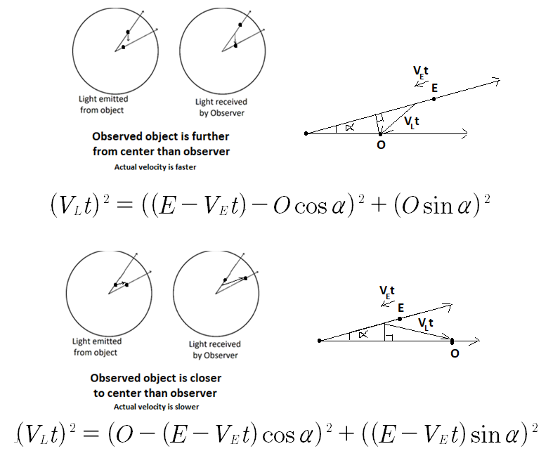
Determining the delay time (t) from emission to observation of the beams of
light.0
α
is the angle from center between the observer and the emitter. :
VL
is the velocity of light (for my model I made it 4,300cm/sec)
VE
is the velocity of the emitter
O
is the distance from center of the Observer at the time of observation
E
is the distance from center of the Emitter at the time of observation
(determined by this expansion motion)
t
= the time required for emitted light to intercept the observer,
and the amount of time that the emitter moved after emission
Solving for t, both equations
reduce to the same solution. This will give me the amount of time the light takes
to travel from the point of emission from its axis to the point it intercepts
the observer on his axis. Solving for t doesn’t matter rather the emitter is
further from center, or closer:

Using my solution for “time for light to
travel”, I populated a new data chart (below). When the chart was complete I
saw that the delay somehow converts the information in the light received to
the Hubble value of the observer, the H at the time of observation (H =
1/observation time). Every object he observed was emitted at different times in
the expansion history, yet it all presents him with the current value of H for
the expansion process. The observer does not have to determine the H value at
the time of emission to analyze his data but can use the current value of H at
the moment the light is received. This was consistent in every scenario I
tried. This new illusion will make the current H value of expansion appear to
be “the” value of H throughout the history of expansion, but it’s not so.
One thing that became clear is that the
delay of observation changes the mechanics of presenting the illusion of center
to the observer. I could no longer draw a “Circle of Observation” around my
observer and then let him watch that circle expand evenly. The observer could
still have such a circle and watch it expand evenly, but the selected objects
that make up that circle would look like a circle only to him. Looking at the
disk from overhead, it would be warped.
This time, I started my disk at 5 seconds
into expansion, and stretched my disk at a rate of 500cm/sec. I placed my
observer at 10,000cm from true center with three objects in a Circle of Observation
around him of radius 866cm. The objects (light emitters) will be in his sky at
60, 90, and 200 degrees from his axis. That means two will be further away
from center than my observer and one closer. I will set the speed of light in
my model to 4,300cm/sec.
Emitter
1: (α = 27.626 degrees Viewer’s angle of 60 degrees is altered
by the delay to 62.3 degrees and it is maintained)
|
Pattern without
Observational Delay
|
Speed of Light
Observational Delay
|
|
Time of
Observation
ta
|
Ha
at Time of
Observation
|
Observer
distance from
center
|
Emitter
distance from
center
at time of Observation
Ea
|
Unmodified
Observed
Distance
Ra
|
tr
Time for
emitted light
to reach Observer
|
Time
Of
Emission
tm
|
HEm
at time of emission
|
Emitter distance
from center
at time of emission
Em
|
Modified
observed
distance
Rm
|
Observer
calculated
Hm
|
|
5sec
|
0.2000000
|
1,000
|
1,617.4
|
866.00
|
0.189
|
4.81
|
0.2078786
|
1,556.10
|
814.90
|
0.2000010
|
|
10sec
|
0.0100000
|
2,000
|
3,234.8
|
17,320.41
|
0.379
|
9.62
|
0.1039397
|
3,112.19
|
1,629.79
|
0.0100005
|
|
5,100sec
|
0.0002000
|
1,020,000
|
1,649,762
|
883,340.73
|
193.303
|
4,906.70
|
0.0002038
|
1,587,231.789
|
831,204.17
|
0.0001961
|
|
15,100sec
|
0.0000662
|
2,020,000
|
4,884,588
|
2,615,381.37
|
572.329
|
14,527.67
|
0.0000688
|
4,699,450.956
|
2,461,016.26
|
0.0000662
|
|
15,095sec
|
|
200cm/sec
|
323.48cm/sec
|
173cm/sec
|
0.03790/sec
|
14,522.86sec
|
|
|
162.98cm/sec
|
|
Observer sees 0.962 seconds of the
emitter motion for every second of his own time. L = 0.962
Emitter
2: (α = 40.893 degrees Viewer’s angle of 90 degrees is altered
by the delay to 93.4 degrees and it is maintained)
|
Pattern without
Observational Delay
|
Speed of Light
Observational Delay
|
|
Time of Observation
ta
|
Ha
at Time of
Observation
|
Observer
distance from
center
|
Emitter
distance from
center
at time of Observation
Ea
|
Unmodified
Observed
Distance
Ra
|
tr
Time for
emitted light
to reach Observer
|
Time
Of
Emission
tm
|
HEm
at time of emission
|
Emitter distance
from center
at time of emission
Em
|
Modified
observed
distance
Rm
|
Observer
calculated
Hm
|
|
5sec
|
0.2000000
|
1,000
|
1,322.85
|
866.00
|
0.197
|
4.80
|
0.2082000
|
1270.74
|
846.85
|
0.1968117
|
|
100sec
|
0.0100000
|
20,000
|
26,457.5
|
17,320.37
|
3.87
|
96.13
|
0.0104030
|
25,432.02
|
1,6667.07cm
|
0.0100000
|
|
5,100sec
|
0.0002000
|
1,020,000
|
1,349,333
|
883,338.93
|
197.68
|
4,902.32
|
0.0002040
|
1,297,033.25
|
850,020.45cm
|
0.0001961
|
|
15,100sec
|
0.0000662
|
3,020,000
|
3,995,085
|
2,615,376.04
|
585.28
|
14,514.72
|
0.0000689
|
3,840,235.71
|
2,516,727.22cm
|
0.0000662
|
|
15,095sec
|
|
200cm/sec
|
264.57cm/sec
|
173.2cm/sec
|
0.03876/sec
|
14,509.92sec
|
|
254.33cm/sec
|
166.67cm/sec
|
|
Observer sees 0.961 seconds of the
emitter motion for every second of his own time. L = 0.961
Emitter
3: (α = 57.845 degrees Viewer’s angle of 200 degrees is altered
by the delay to 199 degrees and it is maintained)
|
Pattern without
Observational Delay
|
Speed of Light
Observational Delay
|
|
Time of
Observation
ta
|
Ha
at Time of
Observation
|
Observer
distance from
center
|
Emitter
distance from
center
at time of Observation
Ea
|
Unmodified
Observed
Distance
Ra
|
tr
Time for
emitted light
to reach Observer
|
Time
Of
Emission
tm
|
HEm
at time of emission
|
Emitter distance
from center
at time of emission
Em
|
Modified
observed
distance
Rm
|
Observer
calculated
Hm
|
|
5sec
|
0.2000000
|
1,000
|
349.85
|
866.00
|
0.202
|
4.80
|
0.2084254
|
335.71
|
869.12
|
0.1926278
|
|
100sec
|
0.0100000
|
20,000
|
6,997.27
|
17,320.53
|
4.035
|
95.97
|
0.0104204
|
6,714.95
|
17,350.19
|
0.0100000
|
|
5,100sec
|
0.0002000
|
1,020,000
|
356,861
|
883,346.87
|
205.781
|
4,894.22
|
0.0002043
|
342,462.48
|
884,859.49
|
0.0001961
|
|
15,100sec
|
0.0000662
|
3,020,000
|
1,056,588
|
2,615,399.55
|
609.274
|
14,490.73
|
0.0000690
|
1,013,957.54
|
2,619,878.11
|
0.0000662
|
|
15,095sec
|
|
200cm/sec
|
69.97cm/sec
|
173.2cm/sec
|
0.0403/sec
|
14,485.93sec
|
|
67.15cm/sec
|
173.50cm/sec
|
|
Observer sees 0.960 seconds of the
emitter motion for every second of his own time. L = 0.96
The light observed was emitted by the object in the past,
and therefore under an older H. Yet, it will present the Hubble Constant Value
at the time of observation. This is true, because the motion of the “image”
presented to the observer is moving in sync for an object that would be
actually at that distance from center at the time of observation and being
observed with no delay. This is always true, so this “phantom” position and
“phantom” motion of the object created by the speed of light is always in sync
with the pattern and will always present the observer with the current H at
time of observation. The delayed observations caused by the speed of light
will not disrupt any of the illusions of this pattern, including the illusion
of center.
The observations delayed by the speed of light alters the
ratio of the distance from center of the observer and the object being
observed. Without the delay of viewing this ratio remained a constant within
this pattern. With the delay it continues to be a constant, but of a different
value.
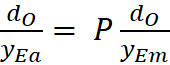
At the moment the light is emitted,  is the correct ratio for the actual
motion of the pair. During the time the emitted light is traveling toward the
observer the observer’s distance from center (new d) is changing but the
Emitter’s (new y) is frozen. Under observational delay this ratio for actual
motion is different than observed motion. This is why θ is altered by the
delay of the speed of light, but since the altered ratio is likewise constant,
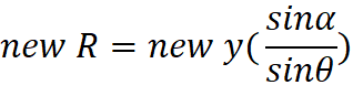
the observed θ is constant. If the delay alters θ then it alters R.
is the correct ratio for the actual
motion of the pair. During the time the emitted light is traveling toward the
observer the observer’s distance from center (new d) is changing but the
Emitter’s (new y) is frozen. Under observational delay this ratio for actual
motion is different than observed motion. This is why θ is altered by the
delay of the speed of light, but since the altered ratio is likewise constant,
the observed θ is constant. If the delay alters θ then it alters R.
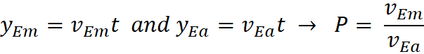
I could see that there is a conversion factor (L) for each
observed object. I found that L can be determined by the observer from his
observed velocity (VRm – velocity at the bottom of the Rm
column) and the speed of light, C (or VL as denoted in my original
equations.)
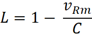
L can also be determined using:
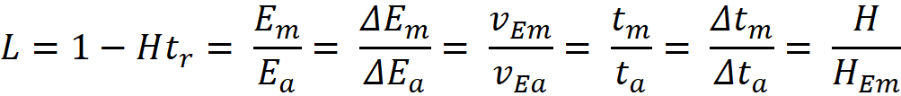
My data charts suggested that the Hubble Constant calculated
by the observer (Hm determined from the delayed observed light), is
the current H (Ha), even though his data is altered by the delayed
observations:
Using the Hubble formula,
VRm = Rm * Hm, since Rm
is the observed distance traveled by the emitted light, then Rm = C
* tr ,
therefore VRm = (C * tr) Hm
If L= 1 – VRm / C , then
L = 1 – Hm * tr
Since the age of expansion when the light was emitted is tm
= ta – tr, then tr = ta - tm,
then;
L = 1 – Hm (ta – tm)
From my formulas for L, tm = L * ta
L = 1 – Hm (ta – L * ta)
L – 1 = Hm * ta (L - 1)
Hm = 1 / ta
Since 1/ta = Ha ,
Hm = Ha
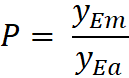
Also, since the ratio of the distance from center before the
delay and after are both constant, then
 where P is a conversion factor
that relates them
where P is a conversion factor
that relates them
Therefore: 
The vector analysis of how light delayed observations
continue to maintain the illusions of center and recession:
Emitter’s perpendicular observed
velocity: Vp = 311.22 * cos(62.3 – 27.626) = 255.95cm/sec
Observer’s projected perpendicular
observed velocity: Vp= - 200 * cos(62.3) = - 92.97cm/sec
Emitter’s tangential observed
velocity: Vt = 311.22 * sin(62.3 – 27.626) = 177.05cm/sec
Observer’s projected tangential
observed velocity: Vt= - 200 * sin(62.3) = - 177.08cm/sec
Just like in the “ideal” pattern (no gravity and no delay),
the observer’s tangential velocities cancel out, even with the altered angle.
The observer still sees the objects moving only directly away from him at the
sum of the perpendiculars…
Vp = 255.95 – 92.97
= 162.98cm/sec
This shows that within this pattern, the illusion of center,
everything receding, is preserved by the speed of light for every observer, and
by the same mechanism of vector interaction. Every observed object will be red
shifted, still.
An illusion of Slow Motion, of time slowed down:
This chart reveals yet another illusion from light delay.
Each successive emission of light takes a little longer than the one before it
to reach the observer. As a result, the passage of time of the emitted object
appears to the observer to move slower. This is true within this pattern
whether he is moving toward the emitted light (closer to center), or away from
it (further out). The result is that the observed emitters in all directions
continue to appear to be receding directly away from the observer with
velocities proportional to distance, but now they are moving in an observed
slow motion.
At each data point, the equations for travel time were used
to move the emitter back down its axis to the point where the light was
emitted. If the observer is looking back toward center, the observed distance
is increased, if toward outer edge, decreased, but regardless of which way he
looks, there is a slowing of motion. For Emitter 1, the delay decreased the
apparent distance traveled by the emitting object on its own axis during the
15,095seconds of observation from the true 4,882,970.60cm to 4,697,894.86cm.
This altered data presents the object as moving only 311.22cm/sec along its
path of motion when it was actually moving 323.48cm/sec.
I wondered how delayed observation would affect measurements
between distant pairs of objects, and would the expansion going on between them
also present the current value of H? Both are viewed from the past, and both
presenting independent delay affects to the observer. The observer’s evaluation
of the relationship between them would be a culmination of these two
independent delays. My first two charts below evaluate the independent
observations of each object, which are then the source of my combined
evaluation of the two together (third chart). I could not perceive how the
observation of the expansion going on between them, measured under all this
noise, might offer the current H to the observer. Turns out, they did, every
time, and it is accomplished by this slowed down observation of distant motion.
I set two new objects in my expanding disk at the 100 second
mark and with expansion of the whole disk still at 500cm/sec. I set the two
objects at the same distance from disk center and at angles of 27.626 degrees
and 32.626 degrees from my observer. This means each will have identical
actual motion away from center, yet each will be viewed differently by my observer
because each will have a different angle α from him. I wanted the two objects to be moving
away from center at a decent velocity, and diverging away from each other at a
moderate expansion velocity. I then let the observer watch them for four
seconds, as he moved along his own axis with expansion motion. What I found is
that the delay still presents the incoming motion as the current H, and it does
so by slowing down the passage of time within the observation, but not in
reality.
Actual motion of expansion between
E1 and E2 (no delays)
|
Time
|
Actual
H
|
α
|
Emitter 1
Actual
Distance from
Center
|
Emitter 2
Actual
Distance from
Center
|
Actual
Distance between
E1 and E2
|
H
between
1 & 2
|
|
100 sec
|
0.01000
|
1.8
|
32,348.30
|
32,348.30
|
2,822.03
|
0.01000
|
|
101 sec
|
0.00990
|
1.8
|
32,671.78
|
32,671.78
|
2,850.25
|
0.00990
|
|
102 sec
|
0.00980
|
1.8
|
32,995.27
|
32,995.27
|
2,878.49
|
0.00980
|
|
103 sec
|
0.00971
|
1.8
|
33,318.75
|
33,318.75
|
2,906.69
|
0.00971
|
|
104 sec
|
0.00961
|
1.8
|
33,642.23
|
33,642.23
|
2,934.91
|
0.00961
|
|
4 sec
|
|
|
323.48cm/sec
|
323.48cm/sec
|
28.22 cm/sec
|
|
Total distance of actual motion
between E1 and E2 during the 4 seconds of observation was
112.88cm at 28.22 cm/sec.
Observed motion of expansion
between E1 and E2 with light delays
|
Time
|
Actual
H
|
Observer’s
Angle of viewing
|
Observed Emitter 1
Offset
position
|
Observed Emitter 2
Offset
position
|
Observed
Distance
between them
|
H btw 1 & 2
Calculated
by
observer
|
|
100 sec
|
0.01000
|
7.6
|
31,122.22
|
31,009.08
|
2,712.89
|
0.01000
|
|
101 sec
|
0.00990
|
7.6
|
31,433.45
|
31,319.17
|
2,740.02
|
0.00990
|
|
102 sec
|
0.00980
|
7.6
|
31,744.67
|
31,629.26
|
2,767.15
|
0.00980
|
|
103 sec
|
0.00971
|
7.6
|
32,055.89
|
31,939.35
|
2,794.27
|
0.00971
|
|
104 sec
|
0.00961
|
7.6
|
32,367.11
|
32,249.44
|
2,821.40
|
0.00961
|
|
4 sec
|
|
|
311.22 cm/sec
|
310.09 cm/sec
|
27.13 cm/sec
|
|
Total distance of observed motion
between E1 and E2 during the 4 seconds of observation was
108.50cm at 27.12 cm/sec.
The delay of receiving the emitted light makes A and E
appear to move in slow motion, but within this the proportional alterations of
velocity and distance corrected the H to the current value at time of observation.
If speed of light delay with the observation of the motion of two objects
moving apart are made to appear to move slower than they really are, then other
actions at a distance would likewise appear so since together they are likewise
diverging. If Emitter 1 were a binary star system rotating around each other
at 3 times per second, my observer should have viewed 12 full rotations, but
instead would have recorded 11.55. If he did not discern this pattern of
motion, he would incorrectly report a rate of 2.89 rotations per second. Every
observation would have a different ratio of time slowdown. If the same binary
pair were at the position of Emitter 2, the observer would report 11.49
rotations at 2.87 rotations per second.
Gravitational
Lensing
I read that scientist were using Gravitational Lensing to
study the expansion rate of the Universe, and that it had confirmed the value
of H offered by recession observations. I looked for raw data to understand
how they were using these observations, but could find only the declaration
that it confirmed current values of H. I decided to build Gravitational
Lensing into my simulator.
To do that, I let the simulator place a “Lensing Object”
between any observer and the object being observed. It halves the angle of
divergence between them (α) and places the Lensing Object at a distance
from center that is the average distance from center of the observer and his
object. The Lensing Object will then be slightly offset from unbent light that
will travel directly to the observer (Fig 1).
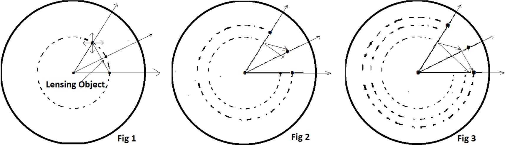
I let my simulator generate a standard data chart with no
lensing. At each pause in my chart, the simulator had moved the Emitter back
toward center to find the point of emission for observed light. For the
Gravitational Lensing simulation, I programmed it to then move all three
objects back to that moment in time (Fig 1). I then built in a sub-simulator
to let the system expand from that moment in the past until the light reached
the Lensing Object (Fig 2). It would then continue until the light reached the
observer (Fig 3).
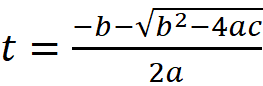
To accomplish this, I had to rework the equations that I had
used to move the Emitter back in time. I needed one that moves the target object
forward in time to the point of interception, (Figs 2 and 3).
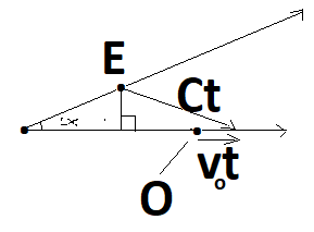

where C is the speed of light

Evaluation
of Light Observed from an Emitting Object at 160,075 Seconds into Expansion
History
I started
the simulation at 1,000 seconds into Expansion (beginning point not shown in
charts):
Observer:
6,000cm from center
Emitting
Object: 6,000cm from center, α=90 degrees
Lensing
Object 1: 6,366cm from center, α=40
degrees
Lensing
Object 2: 5,376cm from center, α=40
degrees
Seed of Light
(C): 200 cm/s
Emitting Object (Undeflected
viewing of emitted light -- shortest possible path to the observer)
|
Expansion
Time at First Observation
|
H at First Observation

|
Observer
Distance
from
Center
|
Emitter
Distance from
Center at time of Observation
α = 90
|
Actual
Distance between
Emitter and
Observer

|
Time for
Emitted Light
To Reach
Observer

|
Expansion Time when Observed light was Emitted
|
H
At time
Observed Light was Emitted
|
Emitter
Distance
From Center
at time of
Emission
|
Distance
Between
Observer
and
Emission
Point at Observation
|
Observer
Calculated
|
|
100,000
|
1.0000E-05
|
600,000.00
|
600,000.00
|
848,528.14
|
4,155.43
|
95,844.57
|
1.0434E-05
|
575,067.44
|
831,085.17
|
1.0000E-05
|
|
150,000
|
6.6667E-06
|
900,000.00
|
900,000.00
|
1,272,792.21
|
6,233.14
|
143,766.86
|
6.9557E-06
|
862,601.17
|
1,246,627.76
|
6.6667E-06
|
|
200,000
|
5.0000E-06
|
1,200,000.00
|
1,200,000.00
|
1,697,056.27
|
8,310.85
|
191,689.15
|
5.2168E-06
|
1,150,134.89
|
1,662,170.35
|
5.0000E-06
|
|
1s/s
|
|
6.00cm/s
|
6.00cm/s
|
8.48cm/s
|
0.0416s/s
|
95,844.58s
0.958s/s
|
|
5.75cm/s
|
vO=8.31cm/s
|
|
L=0.958
Deflecting Object 1 Data
(Deflection and observation of second beam of light, emitted at the same
moment):
|
Expansion Time when Observed light was Emitted
|
Expansion
Time
at
Deflection
|
Deflector
Distance from
Center
at Deflection
|
Time for
Deflected
Light
To reach
Observer

|
Expansion
Time at
Second
(Deflected)
Observation
|
Actual
H
at time of
Second
Observation

|
Observer
Distance from
Center at
Second Observation
|
Distance
Deflected
Light
Traveled
(Perceived Relative Distance)

|
Observer
Calculated
HL

|
Observer
Calculated
HL
|
|
95,844.57
|
98,206.41
|
540,135.25
|
4,322.04
|
100,166.61
|
9.9834E-06
|
600,999.66
|
864,407.10
|
1.0000E-05
|
1.0000E-05
|
|
143,766.86
|
147,309.61
|
810,202.88
|
6,483.05
|
150,249.91
|
6.6556E-06
|
901,499.49
|
1,296,610.64
|
6.6667E-06
|
6.6667E-06
|
|
191,689.15
|
196,412.82
|
1,080,270.51
|
8,644.07
|
200,333.22
|
4.9917E-06
|
1,201,999.32
|
1,728,814.19
|
5.0000E-06
|
5.0000E-06
|
|
|
|
5.50cm/s
|
|
|
|
6.00cm/s
|
Vf =
8.64cm/s
|
|
|
Object 1
Perceived (Projected) Location and Motion (Phantom Object 1)
|
Expansion
Time at
Second
(Deflected)
Observation
|
Actual
H
at time of
Second
Observation
|
Projected Location
of Phantom
Emission Point
(Distance from Center)
dP
|
Phantom
Divergent
Angle
From
Observer

|
Observer
Distance
From
Phantom
Emission
Point
|
Expected Expansion Velocity for an
Object at Projected Distance from Center
( ) )
|
|
100,166.61
|
9.9834E-06
|
785,097.58
|
76.13
|
866,825.49
|
7.84cm/s
|
|
150,249.91
|
6.6556E-06
|
1,177,646.37
|
76.13
|
1,300,238.23
|
7.84cm/s
|
|
200,333.22
|
4.9917E-06
|
1,570,195.16
|
76.13
|
1,733,650.97
|
7.84cm/s
|
|
|
|
7.85cm/s
|
|
8.65cm/s
|
|
Deflecting Object 2 Data
(Deflection and observation of second beam of light, emitted at the same
moment):
|
Expansion Time when Observed light was Emitted
|
Expansion
Time
at
Deflection
|
Deflector
Distance from
Center
at Deflection
|
Time for
Deflected
Light
To reach
Observer
|
Expansion
Time at
Second
(Deflected)
Observation
|
Actual
H
at time of
Second
Observation
|
Observer
Distance from
Center at
Second Observation
|
Distance
Deflected
Light
Traveled
(Perceived Relative Distance)
|
Observer
Calculated
HL
|
Observer
Calculated
HL
|
|
95,844.57
|
98,428.36
|
639,784.37
|
4,682.70
|
100,527.28
|
9.9475E-06
|
603,163.67
|
936,540.80
|
1.0000E-05
|
1.0000E-05
|
|
143,766.86
|
147,642.55
|
959,676.55
|
7,024.06
|
150,790.92
|
6.6317E-06
|
904,745.50
|
1,404,811.20
|
6.6667E-06
|
6.6667E-06
|
|
191,689.15
|
196,856.73
|
1,279,568.73
|
9,365.41
|
201,054.56
|
4.9738E-06
|
1,206,327.34
|
1,873,081.60
|
5.0000E-06
|
5.0000E-06
|
|
|
|
8.50/cm/s
|
|
|
|
6.00cm/s
|
Vf =
9.36cm/s
|
|
|
Object 1
Perceived (Projected) Location and Motion (Phantom Object 1)
|
Expansion
Time at
Second
(Deflected)
Observation
|
Actual
H
at time of
Second
Observation
|
Projected Location
of Phantom
Emission Point
(Distance from Center)
dP
|
Phantom
Divergent
Angle
From
Observer
|
Observer
Distance
From
Phantom
Emission
Point
|
Expected Expansion Velocity for an
Object at Projected Distance from Center
()
|
|
100,527.28
|
9.9475E-06
|
974,331.46
|
68.88
|
943,259.65
|
9.69
|
|
150,790.92
|
6.6317E-06
|
1,461,497.18
|
68.88
|
1,414,889.47
|
9.69
|
|
201,054.56
|
4.9738E-06
|
1,948,662.91
|
68.88
|
1,886,519.29
|
9.69
|
|
|
|
9.69cm/s
|
|
9.38cm/s
|
|
Plot of Data
Charts for Deflecting Object 1:
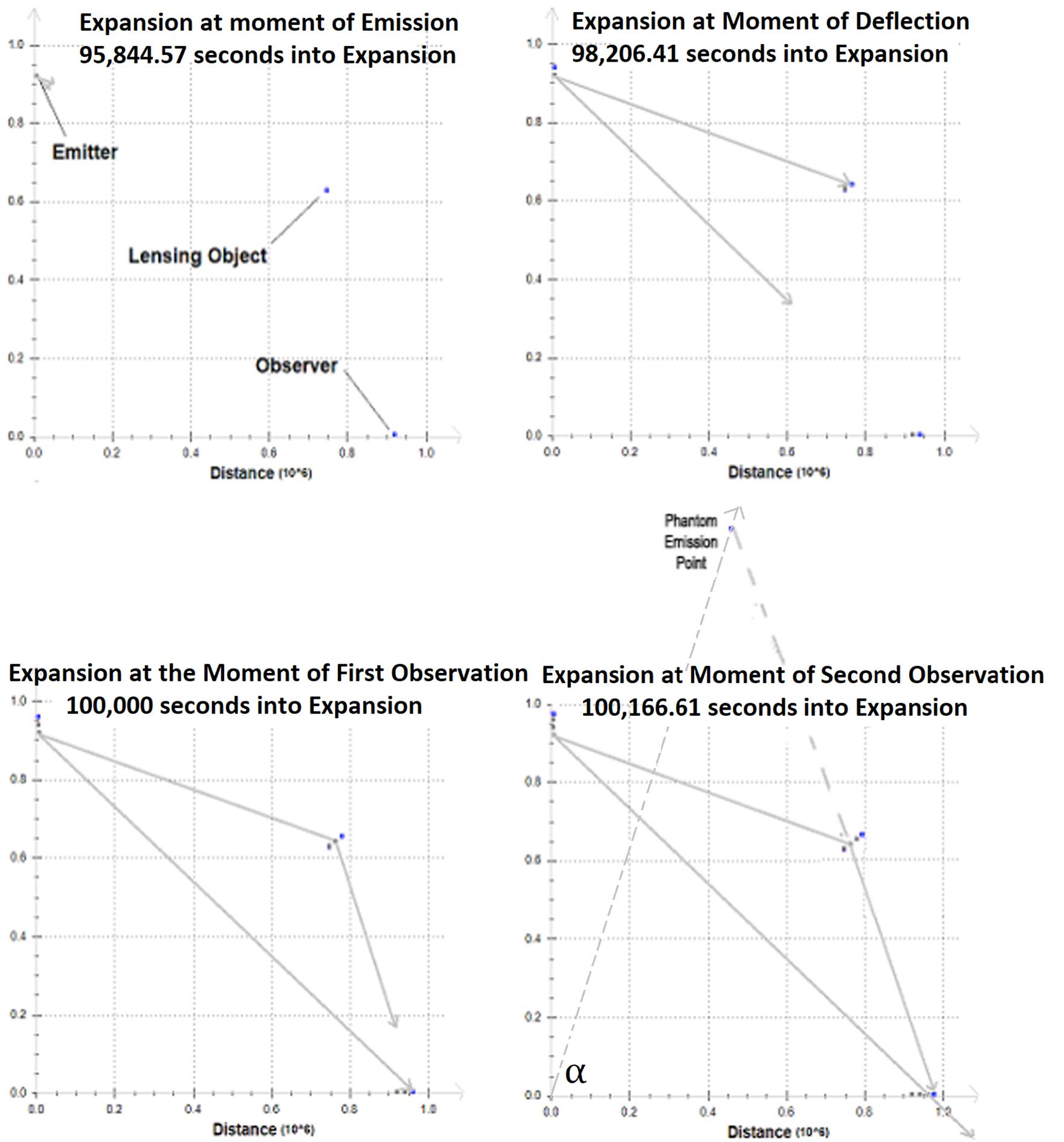
Analysis:
If an emission source were to “flash” on and back off, the
observer could see two (or more) blips of light due to Gravitational Lensing.
There will be an “undeflected” path to every observer, but a few observers will
see the same flash again via deflected light. It appears that using data collected
from those deflected flashes will present the same Hubble Constant Value as the
undeflected observation. This seems true no matter the path and no matter how
many times a flash is deflected. This pattern of Expansion will adjust the
observed (relative) velocity according to the added distance traveled by the
light. This suggests that there are likely stars viewed that are not where
they appear to be, deflections placing them in our sky far from their true
location and motion. From this simulator, it could be that Expansion data
collected from these location illusions will present a calculation of H that is
too high, depending on how long after the first observation is the flash is
seen.
This simulation also suggests that a flash, once
synchronized with the original observation, can be used to calculate the
distance that the light traveled to reach the observer using only the red shift
and the interval between sightings. If so, this would be a way to measure
distances with greater precision, and therefore the Hubble Constant Value.
The difference in speed between the two viewings divided by
the difference in time between the two values times the speed of light, also
provides the H value at the time of unobstructed viewing.
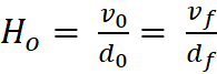
I wondered if this could be used to evaluate the Hubble Constant
Value in terms of directly measured values, Δv and Δt.

Since 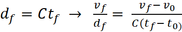
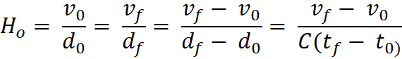
This means you could use Gravitational Lensing to calculate
the distance traveled by the light having any two observations of
simultaneously emitted light that travels different paths to the observer.
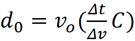 or
or 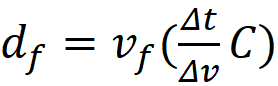
where C is the speed of light
Using observations at 160,075
seconds into expansion to determine the distance traveled by emitted light
around Deflecting Object 1:
If observed light is seen and
sync’ed for unaltered light and Deflecting Object 1

If observed light is seen and
sync’ed for Deflecting Object 2 and Deflecting Object 1

From the Data Chart, the distance
traveled by deflected light around:
Object 1 observed
at 100,167 seconds into expansion was 864,407.0965 cm.
Object 2 observed at 201,054 seconds
into Expansion was 1,873,081.5986cm.
It appears that if you can
observer two beams of light from a specific emitter, with each beam being
emitted at the same moment (sync’ed), no matter the path, you can determine the
distance the light traveled to get to the observer for both paths using only
the red shift of each and the time interval between the two observations. This
could be done with greater precision than H = v/d, where d is an attempt to
measure distance directy.
Speed of
light delay in an accelerating expansion – the H for acceleration is reduced to
the H of steady rate.
(I had to use a computer algorithm to determine “Time for
light to reach Observer”, and I bumped up the speed of light in this simulation
to 300,000cm/s).
.
Example
1: Observer will start at 500cm from center watching an object located at 1,000cm
from center, α = 30 degrees
|
Pattern without
Observational Delay
|
Speed of Light
Observational Delay
|
|
Time of
Observation
|
H
at Time of Observation
2/t
|
Observer
distance from
center
|
Observer
Velocity
|
Emitter
distance from
center
at time of Observation
|
Emitter
Actual
Velocity
|
Distance between Observer
and Object
|
Relative
Velocity
|
Time for
emitted light
to reach observer
|
Emitter distance
from center
at time of emission
|
Actual
Delayed
Velocity
|
Observed
distance
|
Observed
Velocity
|
H
Calculated from observation
v/d
|
H
For a steady
rate expansion
1/t
|
|
10
|
0.200000
|
500
|
100
|
1,000.00
|
200.00
|
619.66
|
123.93
|
0.01
|
999.59
|
149.93
|
619.28
|
92.88
|
0.1499806
|
0.100000
|
|
50
|
0.040000
|
12,500.00
|
500
|
25,000.00
|
1000.00
|
15,491.42
|
619.66
|
0.05
|
24,948.55
|
598.72
|
15,444.35
|
370.63
|
0.0239976
|
0.020000
|
|
100
|
0.020000
|
50,000.00
|
1,000.00
|
100,000.00
|
2,000.00
|
61,965.68
|
1,239.31
|
0.21
|
99,589.82
|
1,194.91
|
61,590.59
|
738.94
|
0.0119976
|
0.010000
|
|
150
|
0.013333
|
112,500.00
|
1,500.00
|
225,000.00
|
3,000.00
|
139,422.79
|
1,858.97
|
0.46
|
223,620.50
|
2,480.61
|
138,161.67
|
1,531.42
|
0.0110843
|
0.006667
|
|
1000
|
0.002000
|
5.000E+06
|
1.000E+04
|
1.000E+07
|
2.000E+04
|
6.197E+06
|
12393.14
|
19.49
|
9.614E+06
|
1.105E+04
|
5.846E+06
|
6.715E+03
|
0.0011487
|
0.001000
|
|
1500
|
0.001333
|
1.125E+07
|
1.500E+04
|
2.250E+07
|
3.000E+04
|
1.394E+07
|
18589.71
|
42.66
|
2.124E+07
|
2.325E+04
|
1.280E+07
|
1.390E+04
|
0.0010865
|
0.000667
|
|
5000
|
0.000400
|
1.250E+08
|
5.000E+04
|
2.500E+08
|
1.000E+05
|
1.549E+08
|
6.197E+04
|
402.050
|
2.114E+08
|
5.434E+04
|
1.206E+08
|
3.080E+04
|
0.0002554
|
0.000200
|
|
50000
|
0.000040
|
1.250E+10
|
5.000E+05
|
2.500E+10
|
1.000E+06
|
1.549E+10
|
6.197E+05
|
36621.630
|
1.790E+09
|
3.508E+04
|
1.099E+10
|
2.415E+05
|
0.0000220
|
0.000020
|
|
|
|
|
10.00cm/s/s
|
|
20.00cm/s/s
|
|
12.39cm/s/s
|
|
|
Decreasing
acceleration
|
|
Decreasing
acceleration
|
|
|
Example 2: Observer will start at 4,000cm from center watching an
object located at 175,500cm from center, α = 30 degrees
|
Pattern without
Observational Delay
|
Speed of Light
Observational Delay
|
|
Time of Observation
|
H
For an accelerating
expansion
|
Observer
distance from
center
|
Observer
Velocity
|
Emitter
distance from
center
at time of Observation
|
Emitter
Actual
Velocity
|
Observed
Distance
|
Relative
Velocity
|
tr
Time for
emitted light
to reach Observer
|
Observed
distance
|
Observed
Velocity
|
Observer
calculated
H
|
H
For a steady
rate expansion
1/t
|
|
10
|
0.200000
|
4,000.00
|
800
|
175,500.00
|
35,100.00
|
172,047.52
|
34,409.50
|
0.51
|
154,444.03
|
21,355.69
|
0.1382746
|
0.100000
|
|
50
|
0.040000
|
100,000.00
|
4,000.00
|
4,387,500.00
|
175,500.00
|
4,301,188.09
|
172,047.52
|
9.37
|
2.811E+06
|
66,413.74
|
0.0236264
|
0.020000
|
|
100
|
0.020000
|
400,000.00
|
8,000.00
|
17,550,000.00
|
351,000.00
|
17,204,752.35
|
344,095.05
|
28.64
|
8.592E+06
|
115,629.02
|
0.0134571
|
0.010000
|
|
500
|
0.004000
|
1.000E+07
|
4.000E+04
|
4.388E+08
|
1.755E+06
|
4.301E+08
|
1.720E+06
|
273.02
|
8.191E+07
|
183,286.60
|
0.0022377
|
0.002000
|
|
1000
|
0.002000
|
4.000E+07
|
8.000E+04
|
1.755E+09
|
3.510E+06
|
1.720E+09
|
3.441E+06
|
641.18
|
1.924E+08
|
220,896.51
|
0.0011484
|
0.001000
|
|
|
|
|
80.00cm/s/s
|
|
3,510.00cm/s/s
|
|
3,440.95cm/s/s
|
|
|
Decreasing
acceleration
|
|
|
As with steady rate expansion, Observers
see a slow motion, but in an accelerating expansion this slowing down of viewed
motion grows slower with time. The conversion constant L is no longer a
constant but changes with time. The speed of light in an accelerating
expansion is disruptive to the perception of Hubble Motion, whereas in steady
rate, it was not.
As with steady rate acceleration,
the motion radio (new d/ new y) is a constant between two objects. Unlike
steady rate, accelerating expansion does not present this ratio as a constant to
the observer who is having to deal with the effects of the speed of light. If
the motion ratio is changing for the observer, θ will be changing for the
observer. The observer will see the object drifting across his sky. (To save
space, I did not include the Emitter distance from Center at time of
observation [new y] after delay or the changing θ.)
These effects on observation caused
by the speed of light diminish with distance. With great distance the rate of
change of the motion ratio as the two diverge away from slows down, becoming
close to a constant again and the drifting across the sky will slow to
unobservable.
Unlike steady rate expansion, at
closer range the H calculated after observational delays is altered to a value that
does not reflect Hubble Motion, a relationship of motions. The observations made
at the same moments (time) in the above charts should offer the same H values
under Hubble Motion, but they don’t. In Example 1 at 10 seconds, H = 0.14998/s.
At the same 10 second moment of expansion Example 2 is H = 0.13827/s. This is
not Hubble motion but just d = v * t. (To me, Hubble motion is simply d = v * t,
but it is more than this and should be expressed differently. Hubble Motion, v
= H * d, expresses a relationship of motions, which is compromised in an
accelerating expansion by the speed of light. Just like with the motion ratio,
this problem diminishes at great distances.
Observed motion begins to return
to a meaningful Hubble relationships at great distances, but with a twist, the
motion begins to look like steady rate expansion. The greater the distance
between objects (therefore the greater the relative velocity), the more speed
of light delays helps accelerating expansion presents itself as steady rate.
At great distances, using actual distances, accelerations, and velocities, H =
2/t, but with observations under the influence of light propagation, H ≃ 1/t, steady rate.
A problem with accelerating
expansion is that actual velocities and relative velocities soon exceed light
speed, and I had to end the simulations not knowing how to proceed. (I never
had to struggle with this under steady rate, except with relative velocities,
which likewise ended my simulations but just meant the objects no longer saw
each other’s light.) But up until those points, as my acceleration simulations
approached these greater distances, the H calculated from observation looked
more and more like the H of steady rate, but were always high. I ran my
simulations out to 20,000 years + and the H calculated seemed to be moving
closer and closer to steady rate values, always high, but never quite got there.
I felt this disproved this pattern as a model, if the expansion in our Universe
is indeed an acceleration, but then I remembered something I had read.
Gravity: Introducing
Relative Acceleration
I knew that so far my simulator was clean motion, that is,
nothing disturbs it. I knew in the real Universe gravity alters motion so I
felt I needed to see how gravity would affect these observations. I knew
gravity causes objects to come together or move together around a Center of
Momentum (CoM). To start incorporating gravity into my simulator I wanted to
know how it would affect two objects moving in this pattern as it pulled them
together. Using the law of Conservation of Momentum, I discovered that as two
objects are being pulled together each object is out-of-sync with the pattern,
but their CoM is always in-sync.
I found that I could place two objects of any mass at
different distances from center, and on the same axis of Expansion Motion, and
their merged positions or orbits would remain in-sync in the pattern. I
determined their velocities based on this pattern, d=vH, and let gravity pull
them towards each other.
Using data from my chart at 100 seconds into expansion (H=.01),
I made the mass of the observer (20,000cm from center, 200cm/sec) to be 100kg.
The emitter (32,348cm from center, 323.48cm/sec) to be 200kg.
CoM = (20,000 * 100 + 32,348 * 200) / (100 + 200) = 28,232cm
from center
Velocity of CoM: (200 * 100 + 323.48 * 200) / (100 + 200) = 282.32cm/sec
If the CoM is located at 28,232cm, the pattern velocity of
my expanding disk would be
Pattern velocity = H * CoM = .01 *
28,232 = 282.32cm/sec
All objects pulled together by gravity eventually merge at
CoM, or circle it. By the Law of Conservation of Momentum, it appears that
gravity will leave common motion in this tiny universe moving in-sync with this
expansion pattern. In other words, the relationships and illusions will be preserved
in some form.
Even if merged masses and masses bound by gravity manage to
stay in-sync, it is certain that an observer would be entangled in an orbit
around a CoM of his own. He is going to be out-of-sync.
I read that earth is part of a super group of galaxies
moving against the CMB at about 600km/sec. Earth is roughly moving 300km/sec.
That could mean that we are being currently slung by our network of orbits in
the opposite direction of the motion of our group (but I could not find any
published data comparing the vector directions). If our super cluster is
moving away from center, then we could be getting slung by our orbit back
toward center at half the speed.
To let my simulator help me examine the possible affects of
the observer and his objects moving out-of-sync, I coded a parameter put the
observer or one of his objects moving too slow or too fast directly away from
center.
I set my observer at 6,000cm from
center and the object being observed at 50,000cm. If in-sync with the pattern,
the Emitter will be moving at 5,000cm/sec away from center and the Observer at
600cm/sec. For the simulation I set the observer out of sync too high and too
low by 300cm/sec.
Scenario
1: α = 45 degrees, all motion in sync
|
Observations
without Light Delay
|
Observations
with Light Delay
|
|
Age of
Expansion
|
H
|
Observer
distance from
center
|
Emitter
Distance from
center
|
Observed
distance
|
Observed
Velocity
|
Time for light
to travel
|
Emitter
Distance from
center at time of emission
|
Observed
Distance
|
Observed
Velocity
|
Calculated
H
|
θ
|
|
|
10
|
0.1000000
|
6,000.00
|
50,000.00
|
45,953.63
|
4,595.36
|
0.15
|
49,246.61
|
45,203.51
|
4,520.35
|
0.1000000
|
50.39
|
|
|
100
|
0.0100000
|
60,000.00
|
500,000.00
|
459,536.28
|
4,595.36
|
1.51
|
492,466.08
|
452,035.08
|
4,520.35
|
0.0100000
|
50.39
|
|
|
50000
|
0.0000200
|
3.00E+07
|
2.50E+08
|
2.30E+08
|
4,595.36
|
7.53E+02
|
2.46E+08
|
2.26E+08
|
4,520.35
|
0.0000200
|
50.39
|
|
|
10000000
|
0.0000001
|
6.00E+09
|
5.00E+10
|
4.60E+10
|
4,595.36
|
1.51E+05
|
4.92E+10
|
4.52E+10
|
4,520.35
|
0.0000001
|
50.39
|
|
|
|
|
600.00cm/sec
|
5,000cm/sec
|
|
4,595.36
|
0.15s/s
|
49,246.61
|
45,203.51
|
4,520.35
|
|
|
|
Scenario 2: α = 45 degrees, Observer is
moving 300cm/sec out of sync too fast
|
Observations
without Light Delay
|
Observations
with Light Delay
|
|
Age of
Expansion
|
H
|
Observer
distance from
center
|
Emitter
Distance from
center
|
Observed
distance
|
Observed
Velocity
|
Time for light
to travel
|
Emitter
Distance from
center at time of emission
|
Observed
Distance
|
Observed
Velocity
|
Calculated
H
|
θ
|
|
10
|
0.1000000000000
|
6,000.00
|
50,000.00
|
45,953.63
|
4,403.78
|
0.1507
|
49,246.61
|
45,203.51
|
4,332.24
|
0.0958385753672
|
50.39
|
|
100
|
0.0100000000000
|
87,000.00
|
500,000.00
|
442,776.14
|
4,409.14
|
1.452
|
492,740.20
|
435,587.92
|
4,337.60
|
0.0099580460911
|
53.12
|
|
1000
|
0.0010000000000
|
897,000.00
|
5,000,000.00
|
4,411,559.95
|
4,409.76
|
14.4666
|
4,927,666.82
|
4,339,990.75
|
4,338.23
|
0.0009995932285
|
53.40
|
|
10000
|
0.0001000000000
|
8.997000E+06
|
5.000000E+07
|
4.409946E+07
|
4,409.77
|
144.6136
|
4.927693E+07
|
4.338408E+07
|
4,338.23
|
0.0000999959457
|
53.43
|
|
50000
|
0.0000200000000
|
4.499700E+07
|
2.500000E+08
|
2.204901E+08
|
4,409.77
|
723.0445
|
2.463848E+08
|
2.169134E+08
|
4,338.23
|
0.0000199998379
|
53.44
|
|
10000000
|
0.0000001000000
|
8.999997E+09
|
5.000000E+10
|
4.409766E+10
|
4,409.77
|
144,607.74
|
4.927696E+10
|
4.338232E+10
|
4,338.23
|
0.0000001000000
|
53.44
|
|
|
|
900.00cm/sec
|
5,000cm/sec
|
|
0.060cm/s/s
|
0.0151s/s
|
|
|
Decreasing
acceleration
|
|
|
Scenario 3: α = 45 degrees, Observer is
moving 300cm/sec out of sync too slow
|
Observations
without Light Delay
|
Observations
with Light Delay
|
|
Age of
Expansion
|
H
|
Observer
distance from
center
|
Emitter
Distance from
center
|
Observed
distance
|
Observed
Velocity
|
Time for light
to travel
|
Emitter
Distance from
center at time of emission
|
Observed
Distance
|
Observed
Velocity
|
Calculated
H
|
θ
|
|
10
|
0.1000000000000
|
6,000.00
|
50,000.00
|
45,953.63
|
4,403.78
|
0.1507
|
49,246.61
|
45,203.51
|
4,332.24
|
0.1030903753679
|
50.39
|
|
100
|
0.0100000000000
|
33,000.00
|
500,000.00
|
477,236.29
|
4,792.03
|
1.5647
|
492,176.30
|
469,422.10
|
4,713.54
|
0.0100411546840
|
47.85
|
|
1000
|
0.0010000000000
|
3.030000E+05
|
5.000000E+06
|
4,790,540.20
|
4,792.56
|
15.707
|
4.921465E+06
|
4.712085E+06
|
4,714.07
|
0.0010004212413
|
47.61
|
|
10000
|
0.0001000000000
|
3.003000E+06
|
5.000000E+07
|
4.79236E+07
|
4,792.57
|
157.1292
|
4.921435E+07
|
4.713876E+07
|
4,714.08
|
0.0001000042216
|
47.58
|
|
50000
|
0.0000200000000
|
1.500300E+07
|
2.500000E+08
|
2.39626E+08
|
4,792.57
|
785.6726
|
2.460716E+08
|
2.357018E+08
|
4,714.08
|
0.0000200001689
|
47.58
|
|
10000000
|
0.0000001000000
|
3.000003E+09
|
5.000000E+10
|
4.79256E+10
|
4,792.57
|
157,135.84
|
4.921432E+10
|
4.714075E+10
|
4,714.08
|
0.0000001000000
|
47.58
|
|
|
|
300.00cm/sec
|
5,000cm/sec
|
|
0.060cm/s/s
|
0.015sec/sec
|
|
|
Decreasing
acceleration
|
|
|
There
were 3 firsts for these simulations:
1.
The
angle of observation (θ) changed with time. From my analysis of the
vector motions to understand how this pattern made every object appear to be
receding from every observer, I could see that for θ to remain constant
the Motion Ratios (new d/ new y) must remain constant. If this pattern is
undisturbed that remains true, but an out of sync situation causes that ratio
to change with time even in the “actual” motion. As a result, θ is
changing, which means objects can now be seen to move across the observer’s sky
within expansion motion. If the altered relative motion is increased by the
out of sync motion, the movement across the sky was clockwise, θ is
decreasing. If it is decreased, it was counterclockwise, θ is increasing.
2.
The
H calculated by the observer was too high or too low, at close range and failed to reflect the
clear relationships of Hubble Motion. This affected faded with distance.
3.
Objects
appeared to the observer to be accelerating. Objects closest to the observer exhibit
the appearance of accelerating. The rate of acceleration decreases with the
distance from observer, in directions, whether the observer is moving too slow
or too fast. This “Relative Acceleration” faded away with distance away from
observer, and is only present in the relative motion between observer and
Emitter. There was no “actual” acceleration in the Expansion Motion of either.
Expansion Acceleration is an illusion.
All three affects diminish with distance away from the
observer, and even go away completely after a certain range. In the many
simulations I ran, this was consistent. The change in the angle  was greatest when objects are closer,
but with distance it also becomes increasingly difficult to see. With distance
the Hubble Constant Value calculated by the observer approaches the correct
value, and the drifting across the sky slows and becomes undetectable.
was greatest when objects are closer,
but with distance it also becomes increasingly difficult to see. With distance
the Hubble Constant Value calculated by the observer approaches the correct
value, and the drifting across the sky slows and becomes undetectable.
The reason the observed object appears to the observer to be
accelerating and moving across the sky, is a disruption in the interaction
between the merged vectors of motion from the two objects, the backbone of the
illusions of all objects receding. Out of sync motion causes the Motion Ratio
(new d/ new y) to change with time.
If altered the velocity of any single object being observed,
that object had its own profile of out of sync motion, but likewise maintained
the appearance of recession and Hubble Motion unless I made the out of syn
extreme.
The
observer’s perspective: a viewed acceleration in steady rate expansion.
I decided to examine a single point in time in the expansion
process using a steady rate expansion, multiple objects at different distances,
and with the observer out of sync.
In the simulations below, I set up an observer and several
objects all at the same distance from center (6000cm) and therefore all moving
the same speed away from center, if all in sync. The first chart represents
all moving in sync with the pattern. I choose 100,000 seconds into expansion as
my observation time; H = .00001/s. Each row of each chart represents a
different object being observed at a different angle α from observer. The
charts that follow it represent out of sync expansions under the same starting
scenario.
Chart 1: Observer and Emitters
at 6,000cm from center, no out of sync motion.
H=.0000100000000/s
|
Α
|
Time for Emitted Light to Reach Observer
|
Observed Distance
|
Observed Velocity
|
Observed
Acceleration
|
Calculated
H
|

|
|
10
|
0.0036
|
1,067.21
|
0.0107
|
0
|
0.0000100000000
|
1.0000000000000
|
|
45
|
0.0155
|
4,662.49
|
0.0469
|
0
|
0.0000100000000
|
1.0000000000000
|
|
70
|
0.0234
|
7,023.38
|
0.0702
|
0
|
0.0000100000000
|
1.0000000000000
|
|
90
|
0.0289
|
8,658.45
|
0.0866
|
0
|
0.0000100000000
|
1.0000000000000
|
|
130
|
0.0370
|
11,097.64
|
0.1110
|
0
|
0.0000100000000
|
1.0000000000000
|
|
160
|
0.0402
|
12,058.87
|
0.1206
|
0
|
0.0000100000000
|
1.0000000000000
|
|
180
|
0.0408
|
12,244.90
|
0.1224
|
0
|
0.0000100000000
|
1.0000000000000
|
Chart 2: Observer and Emitters at
6,000cm from center, Observer out of sync too slow.
H=.0000100000000/s
|
Α
|
Time for Emitted Light to Reach Observer
|
Observed Distance
|
Observed Velocity
|
Observed
Acceleration
|
Calculated
H
|
|
|
10
|
0.0035
|
1,064.47
|
0.0096
|
7.3632E-07
|
0.0000089980515
|
0.8998051542760
|
|
45
|
0.0156
|
4,670.76
|
0.0393
|
1.4435E-07
|
0.0000084210633
|
0.8421063252110
|
|
70
|
0.0233
|
7,000.52
|
0.0588
|
7.5711E-08
|
0.0000084035275
|
0.8403527545570
|
|
90
|
0.0288
|
8,630.21
|
0.0725
|
4.5763E-08
|
0.0000083987158
|
0.8398715792460
|
|
130
|
0.0369
|
11,061.40
|
0.0929
|
1.2754E-08
|
0.0000083950938
|
0.8395093766560
|
|
160
|
0.0401
|
12,019.48
|
0.1009
|
1.9816E-09
|
0.0000083942313
|
0.8394231254310
|
|
180
|
0.0407
|
12,204.90
|
0.1024
|
0.0000E+00
|
0.0000083940874
|
0.8394087352020
|
Chart 3: observer and emitters at
6,000cm, observer moving out of sync too fast.
H=.0000100000000/s
|
α
|
Time for Emitted Light to Reach Observer
|
Observed Distance
|
Observed Velocity
|
Observed
Acceleration
|
Calculated
H
|
|
|
10
|
0.0036
|
1,071.44
|
0.0131
|
7.2794E-07
|
0.0000121881228
|
1.2188122784470
|
|
45
|
0.0157
|
4,701.37
|
0.0546
|
1.4270E-07
|
0.0000116219269
|
1.1621926923980
|
|
70
|
0.0235
|
7,046.40
|
0.0818
|
7.4849E-08
|
0.0000116047190
|
1.1604718976200
|
|
90
|
0.0290
|
8,686.78
|
0.1008
|
4.5241E-08 0
|
0.0000115999971
|
1.1599997050810
|
|
130
|
0.0371
|
11,133.91
|
0.1291
|
1.2609E-08
|
0.0000115964425
|
1.1596442538460
|
|
160
|
0.0403
|
12,098.26
|
0.1403
|
1.9590E-09
|
0.0000115955961
|
1.1595596074170
|
|
180
|
0.0409
|
12,284.90
|
0.1424
|
7.2720E-18
|
0.0000115954548
|
1.1595454847500
|
Plot of Near Objects with Observer Moving Out-of-Sync
(Different data from charts)
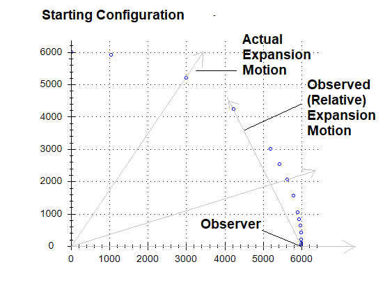
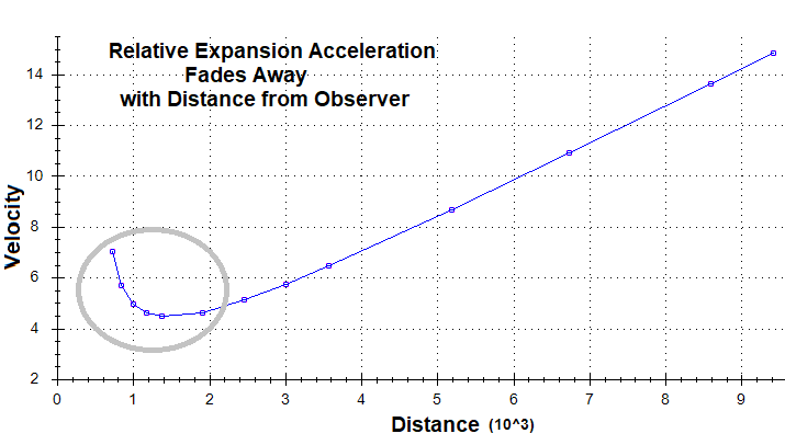
Same Data Points as Objects Move Further Away from Observer
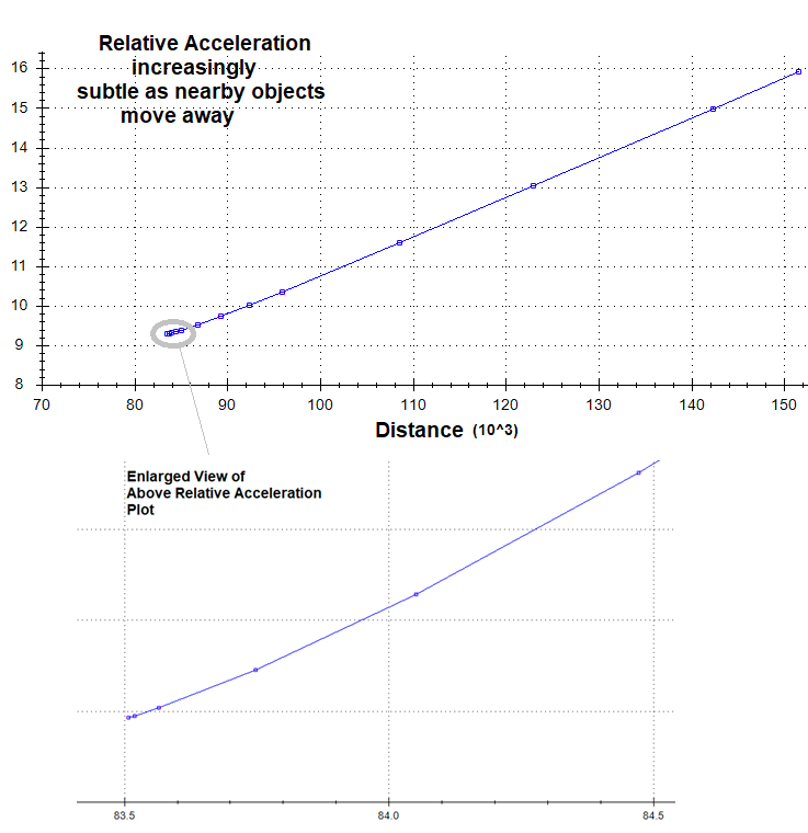
Chart 4: Chart 2 at 6.6 million
years into expansion.
H = 4.76E-18/s
|
α
|
Time for Emitted Light to Reach Observer
|
Observed Distance
|
Observed Velocity
|
Observed
Acceleration
|
Calculated
H
|
|
|
10
|
1.64329E+10
|
4.92986E+15
|
0.0235
|
0
|
4.76191E-18
|
1.0000000000000
|
|
45
|
4.02915E+10
|
1.20875E+16
|
0.0576
|
0
|
4.76191E-18
|
1.0000000000000
|
|
70
|
5.83322E+10
|
1.74997E+16
|
0.0833
|
0
|
4.76191E-18
|
1.0000000000000
|
|
90
|
7.12002E+10
|
2.13601E+16
|
0.1017
|
0
|
4.76191E-18
|
1.0000000000000
|
|
130
|
9.05653E+10
|
2.71696E+16
|
0.1294
|
0
|
4.76191E-18
|
1.0000000000000
|
|
160
|
9.82295E+10
|
2.94688E+16
|
0.1403
|
0
|
4.76191E-18
|
1.0000000000000
|
|
180
|
9.97143E+10
|
2.99143E+16
|
0.1424
|
0
|
4.76191E-18
|
1.0000000000000
|
My simulator could not reduce α significantly to
examine much closer observed distances. In order to see what closer distances
look like I placed my observer at center, set him drifting slightly out of sync
(his velocity within the pattern at center should be zero), and I let him watch
11 objects on the same axis at different distances.
Chart 5: 6.6 million years into
expansion at closer/further observed distances, observer out of sync too slow.
H = 4.76E-18/s
|
Time for Emitted Light to Reach Observer
|
Observed Distance
|
Observed Velocity
|
Observed
Acceleration
|
Calculated
H
|
|
|
0.0633
|
18,992.58
|
9.9965E-14
|
0
|
5.26335E-18
|
1.1053041412590
|
|
0.3085
|
92,545.36
|
4.3447E-13
|
0
|
4.69472E-18
|
0.9858912703770
|
|
3,499.96
|
1.049987E+09
|
5.0073E-09
|
0
|
4.76190E-18
|
0.9999986531220
|
|
34,999,999.95
|
1.050000E+13
|
5.0000E-05
|
0
|
4.76191E-18
|
0.9999999998650
|
|
3.499994E+11
|
1.049998E+17
|
0.50000
|
0
|
4.76191E-18
|
1.0000000000000
|
|
3.442623E+15
|
1.032787E+21
|
4,918.03279
|
0
|
4.76191E-18
|
1.0000000000000
|
|
3.000000E+16
|
9.000000E+21
|
42,857.14286
|
0
|
4.76191E-18
|
1.0000000000000
|
|
1.981132E+17
|
5.943396E+22
|
283,018.86792
|
1.20000E-20
|
4.76191E-18
|
1.0000000000000
|
|
2.087475E+17
|
6.262425E+22
|
298,210.73559
|
2.14500E-18
|
4.76191E-18
|
1.0000000000000
|
|
2.098741E+17
|
6.296222E+22
|
299,820.10791
|
2.04405E-16
|
4.76191E-18
|
0.9999999999990
|
|
2.099874E+17
|
6.299622E+22
|
299,981.99588
|
2.01038E-14
|
4.76191E-18
|
0.9999999981090
|
At this extreme age of expansion, great distances appear to
wash out the out of sync affects, restoring the appearance of clean Hubble
Motion relationships, but closer distances show some distortion. At very close
distances, there is no detectable relative motion. At these closer distances,
with the observer out of sync, the Hubble Values are off, even offering an
appearance within the relative motion of acceleration that increases with
distance. Objects far off wash out the effects from out of sync motion.
I read that the value of H as calculated from observation is
higher than the value derived from the CMB. Since scenario 3 is based motion
from actual calculated motion of earth (and our super cluster) relative to the
CMB, this could suggest that current observations from our expanding Universe
are offering a H that might be high. This model could offer a way to bring
them closer together, suggesting that the value calculated from observations
might be high.
H (derived from observation) = = = 2.33 E -18 /s
H (derived from CMB) = 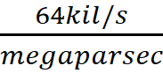 = = 2.07
E -18 /s
= = 2.07
E -18 /s
“Dark
Flow”
NASA reports an observation that suggest a local expansion
within the greater expansion of the cosmos. They named it “dark flow” and have
no explanation for it. Out of sync observation motion within this suggested
pattern produces an observation that sounds much like that. θ changes in
the observer’s sky because his out of sync motion allows him to see the
perpendicular motion vectors. This motion makes his objects move in his sky
(see image below). If he is watching two objects out in front of him, one on
each side of his expansion axis, he will perceive them to be moving away from
each other. He will perceive no cause for this associated with gravity or
expansion motion. It will appear to him to be an expansion within the
expansion. Since distance reduces his observation of θ changing, this
extra motion will appear to be very local and fading away altogether with
distance.
|
|
|
|
|
|
|
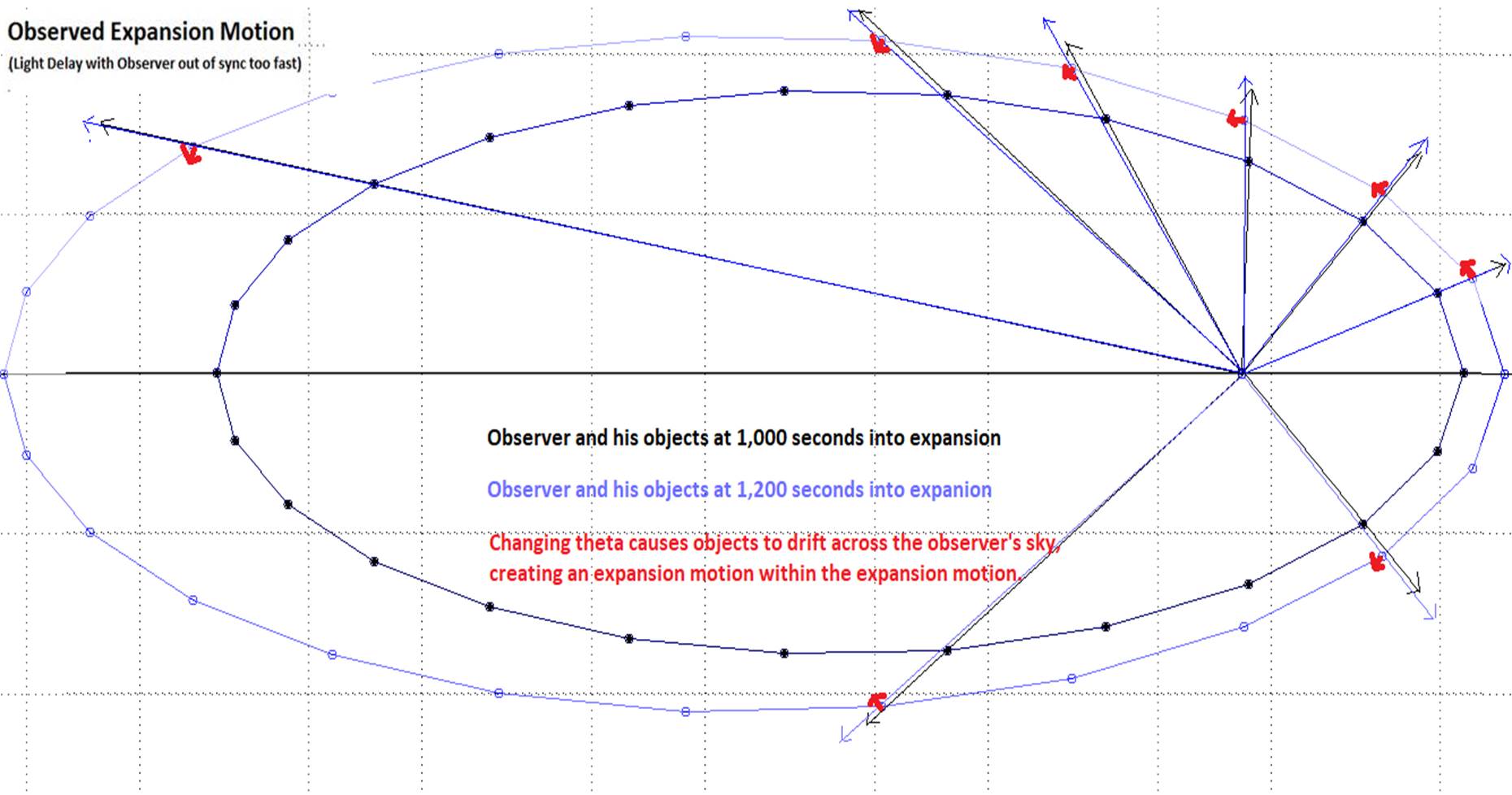
|
|
|
|
|
|
|
|
Observer out of sync too fast
with light speed delays
·
Looking in the direction of expansion motion the observer
will see all objects expanding away from him but they will also appear to be
moving away from his expansion axis, away from each other.
·
In the opposite direction, he will see objects moving towards
his axis, towards each other.
|
Observer out of sync too slow
with light speed delays
·
Looking in the direction of expansion motion the observer
will see all objects expanding away from him but they will also appear to be
moving towards his expansion axis, towards each other.
·
In the opposite direction, he will see objects moving away his
axis, away from each other.
|
|
·
This rate of change of the additional expansion motion will
increase with parpendicular position to his expansion axis, being most
noticible around 60 degrees (with observer moving too fast, around 120 if
moving too slow).
·
With increasing distance from observer, this affect deminishes
and goes away.
·
This expansion within expansion will appear to be “local” in
scope and non-existant at greater distances.
|
I coded my simulator to place objects at near and far
distances from the observer at the same angle in the observer’s sky, and I set
my observer moving out of sync too fast. In other words, I let the observer
stare off into space at a set angle and see objects at different distances (see
data charts below). I wanted to more quantify the shape of the expansion-within-expansion
(“dark flow”) when the observer is moving out of sync. What I could clearly
see is that if the observer is looking in the direction of his motion, the rate
of expansion within expansion will increase with distance away from his axis. In
addition, the closer the object is to him the greater the observed rate of this
expansion away from his axis, with distance this expansion away from his axis
goes away completely, just like relative acceleration. If he looks in the
opposite direction, he will see a contraction toward his axis. However, that
contraction will be much slower, even for objects that are a comparable
distance out in front of him, and therefore the contraction will be more
difficult to see. The rates of expansion and contraction will depend on how
much he is out of sync.
If he is moving too slow, at the same rate he was moving too
fast, the affect is exactly opposite, the data charts are exactly reversed. The
expansion away from his axis will now be happening behind him and at exactly
the rate he would see in front of him if he is moving too fast. The
contraction will now be in front of him and happening at the same much more
subtle rate. His out of sync motion (if along his axis of expansion motion)
will help him locate his axis of motion away form center, but not his direction
along it. He will not be able to tell if he is moving too fast or too slow,
looking toward center or away from it.
|
15 degrees
|
30 degrees
|
60 degrees
|
|
Obj starting at 1,000cm from observer
|
|
t
|
Observed
Distance
|
Observed
θ
|
Δθ
|
|
100
|
999.77
|
15.003
|
|
|
200
|
1,065.75
|
29.058
|
0.14055
|
|
300
|
1,186.75
|
40.864
|
0.11806
|
|
400
|
1,348.04
|
50.173
|
0.09309
|
|
500
|
1,536.99
|
57.347
|
0.07175
|
|
|
Obj starting at 1,000cm from observer
|
|
t
|
Observed
Distance
|
Observed
θ
|
Δθ
|
|
100
|
999.79
|
30.006
|
|
|
200
|
1,239.13
|
53.804
|
0.23798
|
|
300
|
1,614.67
|
68.274
|
0.1447
|
|
400
|
2,053.00
|
76.948
|
0.08674
|
|
500
|
2,521.59
|
82.49
|
0.05542
|
|
|
Obj starting at 1,000cm from observer
|
|
t
|
Observed
Distance
|
Observed
θ
|
Δθ
|
|
100
|
999.87
|
60
|
|
|
200
|
1,732.00
|
90
|
0.30002
|
|
300
|
2,645.78
|
101
|
0.10893
|
|
400
|
3,605.67
|
106
|
0.05209
|
|
500
|
4,582.78
|
109
|
0.03004
|
|
|
|
|
|
|
Obj starting at 4,000cm from observer
|
|
t
|
Observed
Distance
|
Observed
θ
|
Δθ
|
|
100
|
3,998.69
|
15.003
|
|
|
200
|
7,036.55
|
17.111
|
0.02108
|
|
300
|
10,078.19
|
17.947
|
0.00836
|
|
400
|
13,120.97
|
18.396
|
0.00448
|
|
500
|
16,164.26
|
18.675
|
0.00280
|
|
|
Obj starting at 4,000cm from observer
|
|
t
|
Observed
Distance
|
Observed
θ
|
Δθ
|
|
100
|
3,998.77
|
30.006
|
|
|
200
|
7,149.34
|
34.016
|
0.04010
|
|
300
|
10,313.48
|
35.57
|
0.01554
|
|
400
|
13,481.65
|
36.394
|
0.00824
|
|
500
|
16,651.54
|
36.904
|
0.00510
|
|
|
Obj starting at 4,000cm from observer
|
|
t
|
Observed
Distance
|
Observed
θ
|
Δθ
|
|
100
|
3,999.07
|
60
|
|
|
200
|
7,548.23
|
66.6
|
0.06588
|
|
300
|
11,133.26
|
69
|
0.02362
|
|
400
|
14,727.99
|
70.2
|
0.01210
|
|
500
|
18,326.70
|
70.9
|
0.00735
|
|
|
|
|
|
|
Obj starting at 6,000cm from observer
|
|
t
|
Observed
Distance
|
Observed
θ
|
Delta θ
|
|
100
|
5,997.64
|
15.003
|
|
|
200
|
11,032.79
|
16.347
|
0.01344
|
|
300
|
16,070.20
|
16.849
|
0.00502
|
|
400
|
21,108.25
|
17.111
|
0.00262
|
|
500
|
26,146.57
|
17.272
|
0.00161
|
|
|
Obj starting at 6,000cm from observer
|
|
t
|
Observed
Distance
|
Observed
θ
|
Δθ
|
|
100
|
5,997.76
|
30.006
|
|
|
200
|
11,141.09
|
32.578
|
0.02572
|
|
300
|
16,292.69
|
33.525
|
0.00947
|
|
400
|
21,446.59
|
34.016
|
0.00492
|
|
500
|
26,601.46
|
34.318
|
0.00301
|
|
|
Obj starting at 6,000cm from observer
|
|
t
|
Observed
Distance
|
Observed
θ
|
Δθ
|
|
100
|
5,998.20
|
60
|
|
|
200
|
11,529.26
|
64.3
|
0.04308
|
|
300
|
17,083.21
|
65.8
|
0.01511
|
|
400
|
22,643.21
|
66.6
|
0.00769
|
|
500
|
28,205.67
|
67.1
|
0.00466
|
|
|
|
|
|
|
Obj starting at 10,000cm from observer
|
|
t
|
Observed
Distance
|
Observed
θ
|
Δθ
|
|
100
|
9,994.74
|
15.003
|
|
|
200
|
19,025.83
|
15.782
|
0.00779
|
|
300
|
28,058.18
|
16.060
|
0.00278
|
|
400
|
37,090.86
|
16.202
|
0.00142
|
|
500
|
46,123.69
|
16.289
|
0.00087
|
|
|
Obj starting at 10,000cm from observer
|
|
t
|
Observed
Distance
|
Observed
θ
|
Δ
|
|
100
|
9,994.94
|
30.006
|
0
|
|
200
|
19,130.87
|
31.503
|
0.01498
|
|
300
|
28,271.42
|
32.033
|
0.00529
|
|
400
|
37,413.20
|
32.303
|
0.00271
|
|
500
|
46,555.50
|
32.468
|
0.00164
|
|
|
Obj starting at 10,000cm from observer
|
|
t
|
Observed
Distance
|
Observed
θ
|
Δθ
|
|
100
|
9,995.67
|
60.00
|
|
|
200
|
19,510.93
|
62.60
|
0.02544
|
|
300
|
29,039.42
|
63.40
|
0.00875
|
|
400
|
38,571.34
|
63.90
|
0.00443
|
|
500
|
48,104.65
|
64.10
|
0.00267
|
|
|
|
|
|
|
Obj starting at 40,000cm from observer
|
|
t
|
Observed
Distance
|
Observed
θ
|
Δθ
|
|
100
|
39,939.03
|
15.00
|
|
|
200
|
78,914.05
|
15.19
|
0.0019
|
|
300
|
117,889.35
|
15.26
|
0.0006
|
|
400
|
156,864.73
|
15.29
|
0.0003
|
|
500
|
195,840.13
|
15.31
|
0.0002
|
|
|
Obj starting at 40,000cm from observer
|
|
t
|
Observed
Distance
|
Observed
θ
|
Δθ
|
|
100
|
39,939.83
|
30.01
|
|
|
200
|
79,016.57
|
30.37
|
0.0036
|
|
300
|
118,094.37
|
30.49
|
0.0012
|
|
400
|
157,172.45
|
30.55
|
0.0006
|
|
500
|
196,250.63
|
30.59
|
0.0004
|
|
|
Obj starting at 40,000cm from observer
|
|
t
|
Observed
Distance
|
Observed
θ
|
Δθ
|
|
100
|
39,942.75
|
60.00
|
|
|
200
|
79,391.08
|
60.60
|
0.00625
|
|
300
|
118,842.58
|
60.80
|
0.00210
|
|
400
|
158,294.89
|
61.00
|
0.00105
|
|
500
|
197,747.51
|
61.00
|
0.00063
|
|
|
|
|
|
|
Obj starting at 80,000cm from observer
|
|
t
|
Observed
Distance
|
Observed
θ
|
Δθ
|
|
100
|
79,771.86
|
15.00
|
|
|
200
|
158,580.78
|
15.10
|
0.0009
|
|
300
|
237,389.84
|
15.13
|
0.0003
|
|
400
|
316,198.93
|
15.14
|
0.0002
|
|
500
|
395,008.04
|
15.15
|
9E-05
|
|
|
Obj starting at 80,000cm from observer
|
|
t
|
Observed
Distance
|
Observed
θ
|
Δθ
|
|
100
|
79,773.45
|
30.01
|
|
|
200
|
158,684.17
|
30.19
|
0.0018
|
|
300
|
237,595.41
|
30.25
|
0.0006
|
|
400
|
316,506.79
|
30.28
|
0.0003
|
|
500
|
395,418.22
|
30.30
|
0.0002
|
|
|
Obj starting at 80,000cm from observer
|
|
t
|
Observed
Distance
|
Observed
θ
|
Δθ
|
|
100
|
79,779.28
|
60.00
|
|
|
200
|
159,062.44
|
60.30
|
0.00312
|
|
300
|
238,347.17
|
60.40
|
0.00104
|
|
400
|
317,632.30
|
60.50
|
0.00052
|
|
500
|
396,917.58
|
60.50
|
0.00031
|
|
|
|
|
|
|
Obj starting at 10,000,000cm from observer
|
|
t
|
Observed
Distance
|
Observed
θ
|
Δθ
|
|
100
|
967,561.05
|
15.00
|
|
|
200
|
1,934,187.53
|
15.00
|
0
|
|
300
|
2,900,814.03
|
15.00
|
0
|
|
400
|
3,867,440.53
|
15.00
|
0
|
|
500
|
4,834,067.03
|
15.00
|
0
|
|
|
Obj starting at 10,000,000cm from observer
|
|
t
|
Observed
Distance
|
Observed
θ
|
Δθ
|
|
100
|
967,579.76
|
30.006
|
|
|
200
|
1,934,321.68
|
30.021
|
0.00015
|
|
300
|
2,901,063.64
|
30.025
|
0.00005
|
|
400
|
3,867,805.61
|
30.028
|
0.00002
|
|
500
|
4,834,547.58
|
30.029
|
0.00001
|
|
|
Obj starting at 10,000,000cm from observer
|
|
t
|
Observed
Distance
|
Observed
θ
|
Δθ
|
|
100
|
967,648.31
|
60.010
|
|
|
200
|
1,934,813.12
|
60.036
|
0.00026
|
|
300
|
2,901,978.06
|
60.044
|
0.00009
|
|
400
|
3,869,143.03
|
60.048
|
0.00004
|
|
500
|
4,836,308.02
|
60.051
|
0.00003
|
|
|
120 degrees
|
150 degrees
|
165 degrees
|
|
Obj starting at 1,000cm from observer
|
|
t
|
Observed
Distance
|
Observed
θ
|
Δθ
|
|
100
|
1,000.07
|
120.010
|
|
|
200
|
2,646.07
|
139.115
|
0.19105
|
|
300
|
4,359.47
|
143.421
|
0.04306
|
|
400
|
6,083.58
|
145.292
|
0.01872
|
|
500
|
7,811.32
|
146.337
|
0.01044
|
|
|
Obj starting at 1,000cm from observer
|
|
t
|
Observed
Distance
|
Observed
θ
|
Δθ
|
|
100
|
1,000.14
|
150.006
|
|
|
200
|
2,909.76
|
159.900
|
0.09895
|
|
300
|
4,837.32
|
161.936
|
0.02036
|
|
400
|
6,767.51
|
162.812
|
0.00875
|
|
500
|
8,698.57
|
163.298
|
0.00487
|
|
|
Obj starting at 1,000cm from observer
|
|
t
|
Observed
Distance
|
Observed
θ
|
Δθ
|
|
100
|
1,000.16
|
165.003
|
|
|
200
|
2,977.68
|
169.989
|
0.04986
|
|
300
|
4,959.76
|
170.994
|
0.01004
|
|
400
|
6,942.48
|
171.424
|
0.00431
|
|
500
|
8,925.43
|
171.664
|
0.00239
|
|
|
|
|
|
|
Obj starting at 4,000cm from observer
|
|
t
|
Observed
Distance
|
Observed
θ
|
Δθ
|
|
100
|
3,999.87
|
120.01
|
|
|
200
|
8,543.87
|
125.828
|
0.05818
|
|
300
|
13,114.74
|
127.599
|
0.01772
|
|
400
|
17,691.67
|
128.455
|
0.00855
|
|
500
|
22,270.92
|
128.958
|
0.00504
|
|
|
Obj starting at 4,000cm from observer
|
|
t
|
Observed
Distance
|
Observed
θ
|
Δθ
|
|
100
|
4,000.16
|
150.006
|
|
|
200
|
8,880.52
|
153.233
|
0.03228
|
|
300
|
13,769.06
|
154.171
|
0.00937
|
|
400
|
18,659.36
|
154.617
|
0.00446
|
|
500
|
23,550.32
|
154.877
|
0.00261
|
|
|
Obj starting at 4,000cm from observer
|
|
t
|
Observed
Distance
|
Observed
θ
|
Δθ
|
|
100
|
4,000.24
|
165.003
|
|
|
200
|
8,970.21
|
166.656
|
0.01653
|
|
300
|
13,942.33
|
167.131
|
0.00474
|
|
400
|
18,914.89
|
167.356
|
0.00225
|
|
500
|
23,887.63
|
167.487
|
0.00131
|
|
|
|
|
|
|
Obj starting at 4,000cm from observer
|
|
t
|
Observed
Distance
|
Observed
θ
|
Δθ
|
|
100
|
99,677.71
|
120.01
|
|
|
200
|
199,855.83
|
120.258
|
0.00248
|
|
300
|
300,035.19
|
120.341
|
0.00082
|
|
400
|
400,214.86
|
120.382
|
0.00041
|
|
500
|
500,394.66
|
120.407
|
0.00025
|
|
|
Obj starting at 1,000,000cm from observer
|
|
t
|
Observed
Distance
|
Observed
θ
|
Δθ
|
|
100
|
967,904.18
|
150.006
|
|
|
200
|
1,936,646.70
|
150.021
|
0.00015
|
|
300
|
2,905,389.26
|
150.025
|
0.00005
|
|
400
|
3,874,131.83
|
150.028
|
0.00002
|
|
500
|
4,842,874.40
|
150.029
|
0.00001
|
|
|
Obj starting at 1,000,000cm from observer
|
|
t
|
Observed
Distance
|
Observed
θ
|
Δθ
|
|
100
|
967,922.89
|
165.003
|
|
|
200
|
1,936,780.76
|
165.011
|
0.00008
|
|
300
|
2,905,638.63
|
165.013
|
0.00003
|
|
400
|
3,874,496.51
|
165.014
|
0.00001
|
|
500
|
4,843,354.39
|
165.015
|
0.00001
|
|
Out of
Sync Gravitational Lensing
When everything was in sync, Gravitational Lensing generated
the same H for all lensed light as if it were not lensed. The raw data, speed
and distance reflected the alteration, but the H they produced was the same.
This is not so if the observer is out of sync. But, as separation grows, the
effect of the out of sync goes away, Gravitational Lensing returns to offering
the same H for all light emitted by the observed object, lensed or not.
The results remain consistent with past simulations; if the
observer is out of sync too slow, the H value calculated by the observer is low
compared to the actual expansion value at the time of observation but becomes
accurate at greater distances. If too high, the H calculated is high, but
becomes accurate with greater distances.
Initial Observation Chart:
Observation of Light Traveling directly from Emitting Object to Observer with
Observer out of sync too slow
|
Expansion
Time at First Observation
|
H at First Observation
|
Observer
Distance
from
Center
|
Emitter
Distance from
Center α = 70
|
Time for
Light to
Reach
Observer
|
Observed
Distance
|
Emitter
Distance at time of Emission
|
Observed
Velocity

|
Observed
Acceleration
|
Observer
Calculated
|
|
100,000
|
0.0000100000000
|
6,062.45
|
6,122.45
|
0.02329714
|
6,989.14
|
6,122.45
|
0.05320224
|
2.521688E-07
|
0.0000076085184
|
|
100,100
|
0.0000099900100
|
6,065.57
|
6,128.57
|
0.02331488
|
6,994.46
|
6,128.57
|
0.05321060
|
8.360912E-08
|
0.0000076063364
|
|
100,200
|
0.0000099800399
|
6,068.69
|
6,134.69
|
0.02333261
|
6,999.78
|
6,134.69
|
0.05321894
|
8.341860E-08
|
0.0000076017487
|
|
100,300
|
0.0000099700897
|
6,071.82
|
6,140.82
|
0.02335035
|
7,005.11
|
6,140.81
|
0.05322726
|
8.322862E-08
|
0.0000075971643
|
|
100,400
|
0.0000099601594
|
6,074.94
|
6,146.94
|
0.02336809
|
7,010.43
|
6,146.94
|
0.05844419
|
2.500000E-20
|
0.0000075925833
|
|
2.100000E+17
|
4.761905E-18
|
6.557143E+15
|
1.2857142857E+16
|
40,910,934,093
|
1.2273280228E+16
|
1.2857140352E+16
|
0.05844419
|
0
|
4.76190500E-18
|
|
2.200000E+17
|
4.545455E-18
|
6.869388E+15
|
1.3469387755E+16
|
42,859,073,812
|
1.2857722144E+16
|
1.3469385131E+16
|
0.05844419
|
0
|
4.54545500E-18
|
|
2.300000E+17
|
4.347826E-18
|
7.181633E+15
|
1.4081632653E+16
|
44,807,213,531
|
1.3442164059E+16
|
1.4081629910E+16
|
0.05844419
|
0
|
4.34782600E-18
|
|
2.400000E+17
|
4.166667E-18
|
7.493878E+15
|
1.4693877551E+16
|
46,755,353,250
|
1.4026605975E+16
|
1.4693874688E+16
|
0.05844419
|
0
|
4.16666700E-18
|
|
2.500000E+17
|
4.000000E-18
|
7.806122E+15
|
1.5306122449E+16
|
48,703,492,968
|
1.4611047891E+16
|
1.5306119467E+16
|
0.05844419
|
0
|
4.00000000E-18
|
Secondary Observation Chart:
Observation of Light Emitted at the same moment traveling from Emitting Object,
around Lensing Object, to Observer who is out of sync to slow
|
Expansion
Time at First Observation
|
H
at First Observation
|
Expansion
Time at Second Observation
|
H
at Second Observation
|
Time for Light to Reach Observer
|
Distance
Light
Traveled
|
Observed
Velocity

|
Observer
Calculated
H
|
Observer
Calculated
H
|
|
100,000
|
0.0000100000000
|
100,000.02
|
0.0000099999976
|
0.02448876
|
7,346.63
|
0.06507526
|
0.0000088489689
|
0.0000331008736
|
|
100,100
|
0.0000099900100
|
100,100.02
|
0.0000099900075
|
0.02451045
|
7,353.13
|
0.06509687
|
0.0000088500024
|
0.0000331027310
|
|
100,200
|
0.0000099800399
|
100,200.02
|
0.0000099800375
|
0.02453215
|
7,359.64
|
0.06511843
|
0.0000088451108
|
0.0000330302118
|
|
100,300
|
0.0000099700897
|
100,300.02
|
0.0000099700873
|
0.02455385
|
7,366.16
|
0.06513994
|
0.0000088402186
|
0.0000329579641
|
|
100,400
|
0.0000099601594
|
100,400.02
|
0.0000099601569
|
0.02457557
|
7,372.67
|
0.07671415
|
0.0000088353257
|
0.0000328859862
|
|
2.100000E+17
|
4.761905E-18
|
2.10000054E+17
|
4.76190400E-18
|
5.369991E+10
|
1.610997E+16
|
0.07671415
|
4.761905E-18
|
4.761905E-18
|
|
2.200000E+17
|
4.545455E-18
|
2.20000056E+17
|
4.54545300E-18
|
5.625704E+10
|
1.687711E+16
|
0.07671415
|
4.545455E-18
|
4.545455E-18
|
|
2.300000E+17
|
4.347826E-18
|
2.30000059E+17
|
4.34782500E-18
|
5.881418E+10
|
1.764425E+16
|
0.07671415
|
4.347826E-18
|
4.347826E-18
|
|
2.400000E+17
|
4.166667E-18
|
2.40000061E+17
|
4.16666600E-18
|
6.137132E+10
|
1.841140E+16
|
0.07671415
|
4.166667E-18
|
4.166667E-18
|
|
2.500000E+17
|
4.000000E-18
|
2.50000064E+17
|
3.99999900E-18
|
6.392846E+10
|
1.917854E+16
|
0.07671415
|
4.000000E-18
|
4.000000E-18
|
Where subscript “f” is values from the second observation,
and “o” is from the first
Orbital
Out of Sync Motion
Above, I explored “out of sync motion” by setting the
observer out of sync with the overall expansion motion with the observer moving
directly away from center. I had explored the idea that Conservation of Momentum
(COM), mass clumps moving together, might be what is moving in sync with the
pattern, not the observer. The observer would be in orbit around his COM.
Likewise, the objects he is observer would be in orbit around their COM. The
observer and the objects being observed would not be in sync but held close to
in-sync by their COM’s. I decided to write another simulator to move COM
points away from center in this Expansion pattern, instead of objects, and added
code to a single object in orbit around each (the observer included).
To do that, I added parameters to each point (COM) moving
away from center to describe an object moving in a circle around it. For each
object, these parameters could alter the radius of orbit, the time it takes to
complete a single orbit, and a starting angle of orbit measured from the COM’s
axis of motion. For my first simulation, I created 13 COM points with orbital
parameters manually chosen at random. When I plotted the results, it looked
familiar, like charts I see every time I google “Hubble Value”.
A Sample Chart from the Webb:
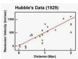
Configuration
of My Manually Selected Random Objects
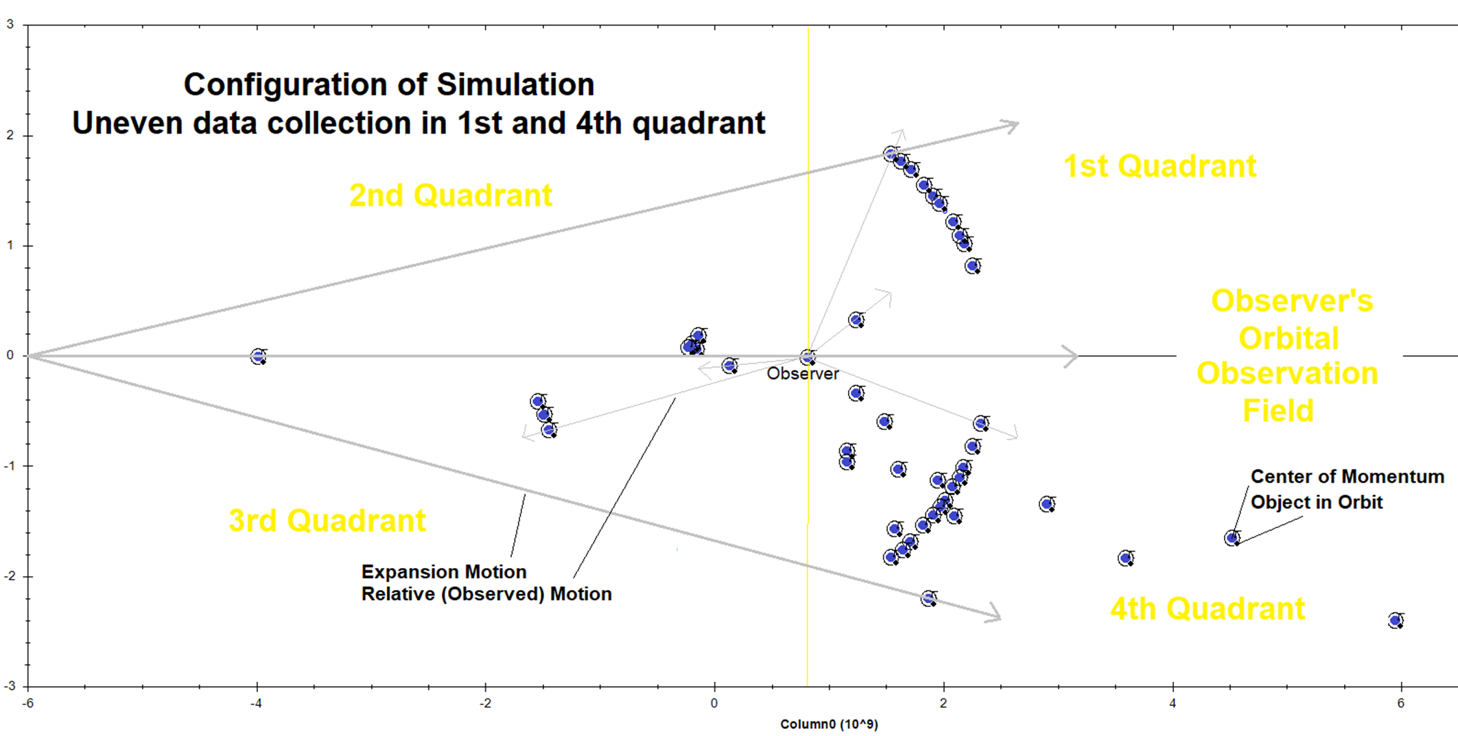
In these charts, the COM’s are moving away from center
in-sync with this Expansion Motion pattern. Each has an object orbiting (one
is the observer). But, the out of sync motion is held in check within the
pattern by its COM.
My Initial
Charts:
Data Chart 1 – Several objects are observed Blue
Shifted
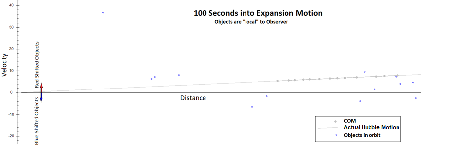
Data Chart 2 – All objects observed Red Shifted
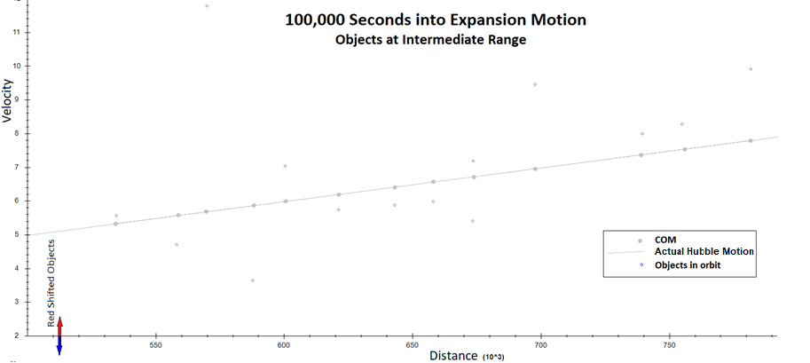
Data Chart 3 – All objects observed Red Shifted
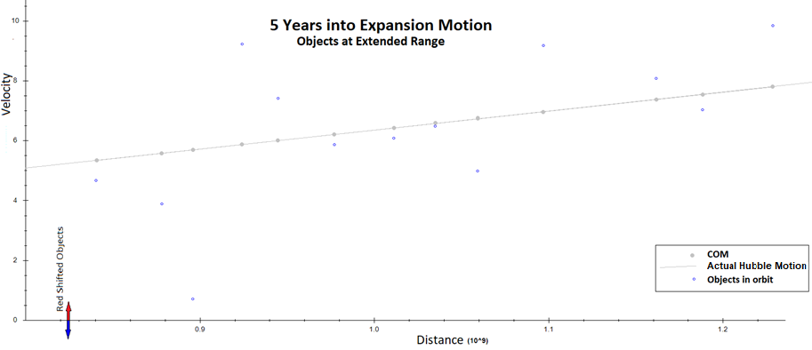
When I averaged the Hubble Constant Values calculated from
each object being observed, the value was consistently high. When I thought
about it, I could see how the orbits could create this problem, especially
seeing how lopsided I had created the distribution of COM’s around the observer’s
COM.
I ran another simulation with just two objects for the
observer. Each object’s COM was the same distance from the observer’s COM, 180
degrees apart, and with all orbits the same radius and in sync. When the
Expanison was young, this configuration gave the observer an accurate Hubble
Constant Value with a percent error of 0.00% and in all positions of the
observer’s orbit around his COM. The error increased to 2.70% as the Expansion
age reached 1 billion years. The2 .7% was consistent consistent all the way
around the observer’s orbit. It was clear to me that two objects 180 degrees
apart, with their distances from their respective COMs to the observer’s COM
being equal, and orbits in sync, offered an offset of the errors introduced by
the observer’s orbit.
I let my simulator generate evenly distributed COM/object
pairs in circles around my observer and his COM. I left all orbits in sync and
the same radius. I then ran multiple simulations with the observer’s starting
orbital angles off his COM’s axis away from center to 0, 90, 180, and 270
degrees.
Evenly Spaced COMs around the Observer and His COM
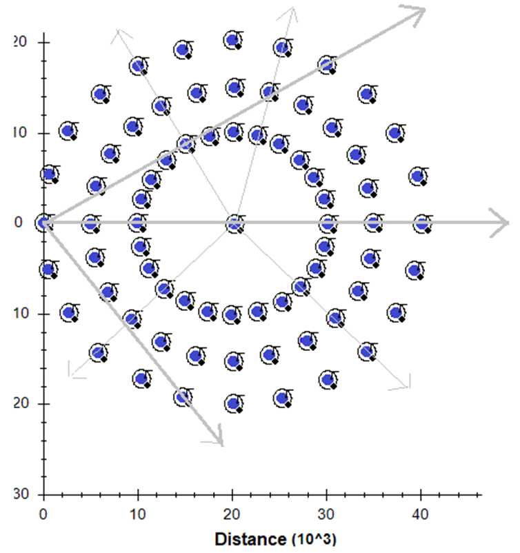
In the early stages of Expansion for this configuration, the
average H was accurate to within 0.0% As the Expansion aged the accuracy dropped,
but after 1 million years it only dropped to about 3%, comparable to watching
just two objects of perfect placement. What was most different was that the
observer calculated a large range of individual H values that averaged out the
errors caused by the observer’s orbit. The result was an accurate Hubble
Constant Value, no matter what quadrant the observer was in around his COM. I
let the age of Expansion go out to 1 billion years.
Lopsided
Configuration of Many Objects
I set up the simulator to again generate many COM/object
pairs around my observer’s COM. This time, I let it place the pairs unevenly
in different quadrants.
Observer Moving in First Quadrant of His Orbit Around His
Center of Momentum
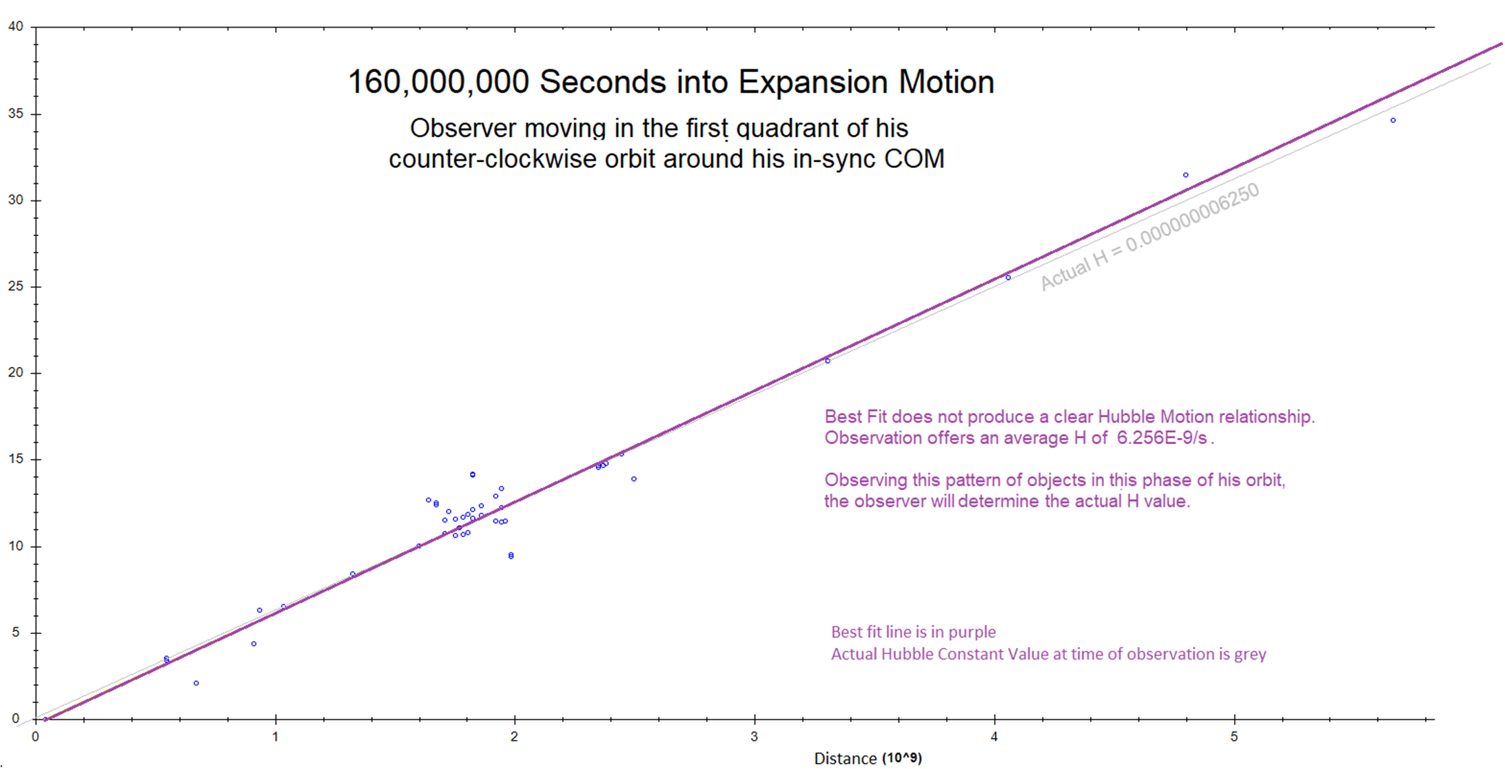
Observer Moving in Second Quadrant of His Orbit Around His
Center of Momentum
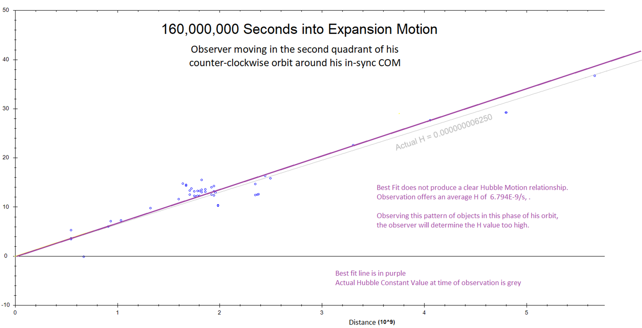
Observer Moving in Third Quadrant of His Orbit Around His
Center of Momentum
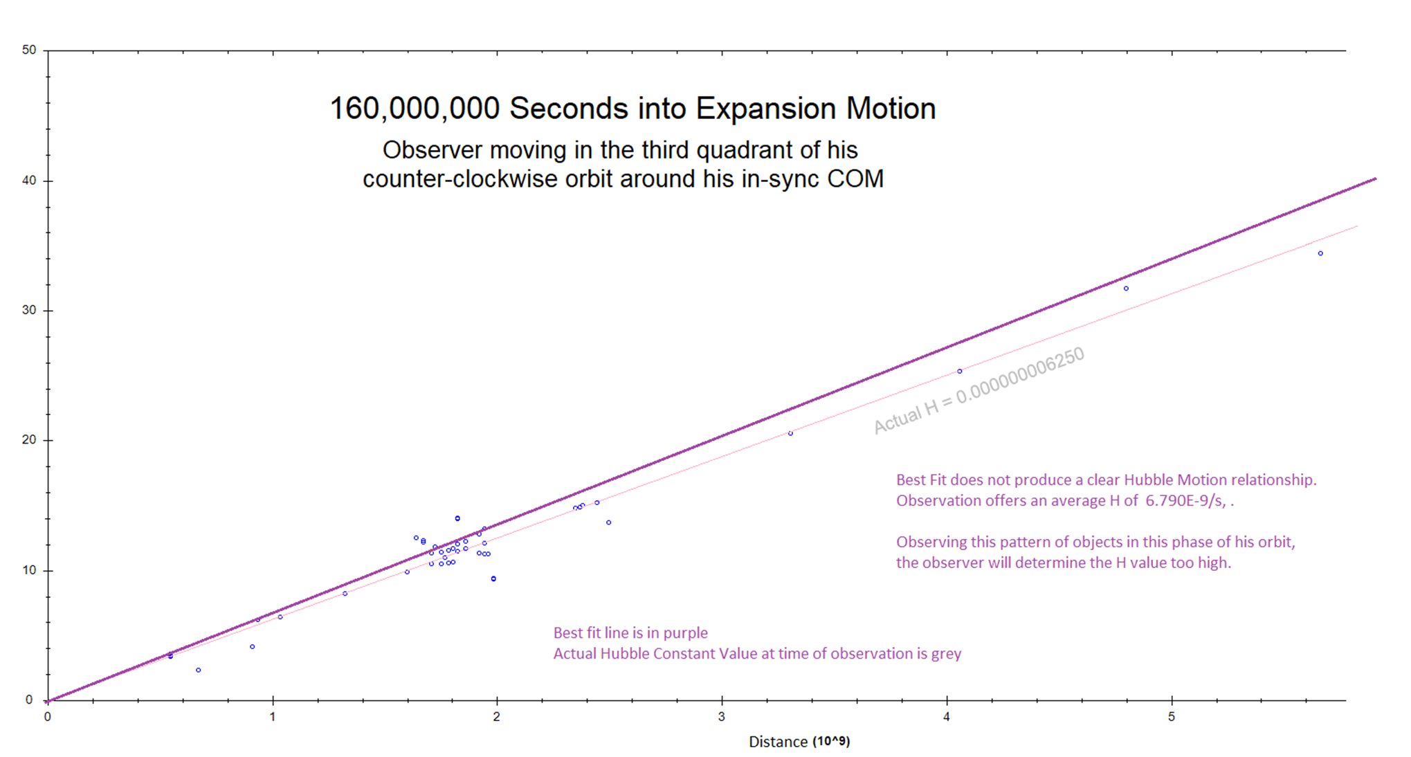
Observer Moving in Third Quadrant of His Orbit Around His
Center of Momentum
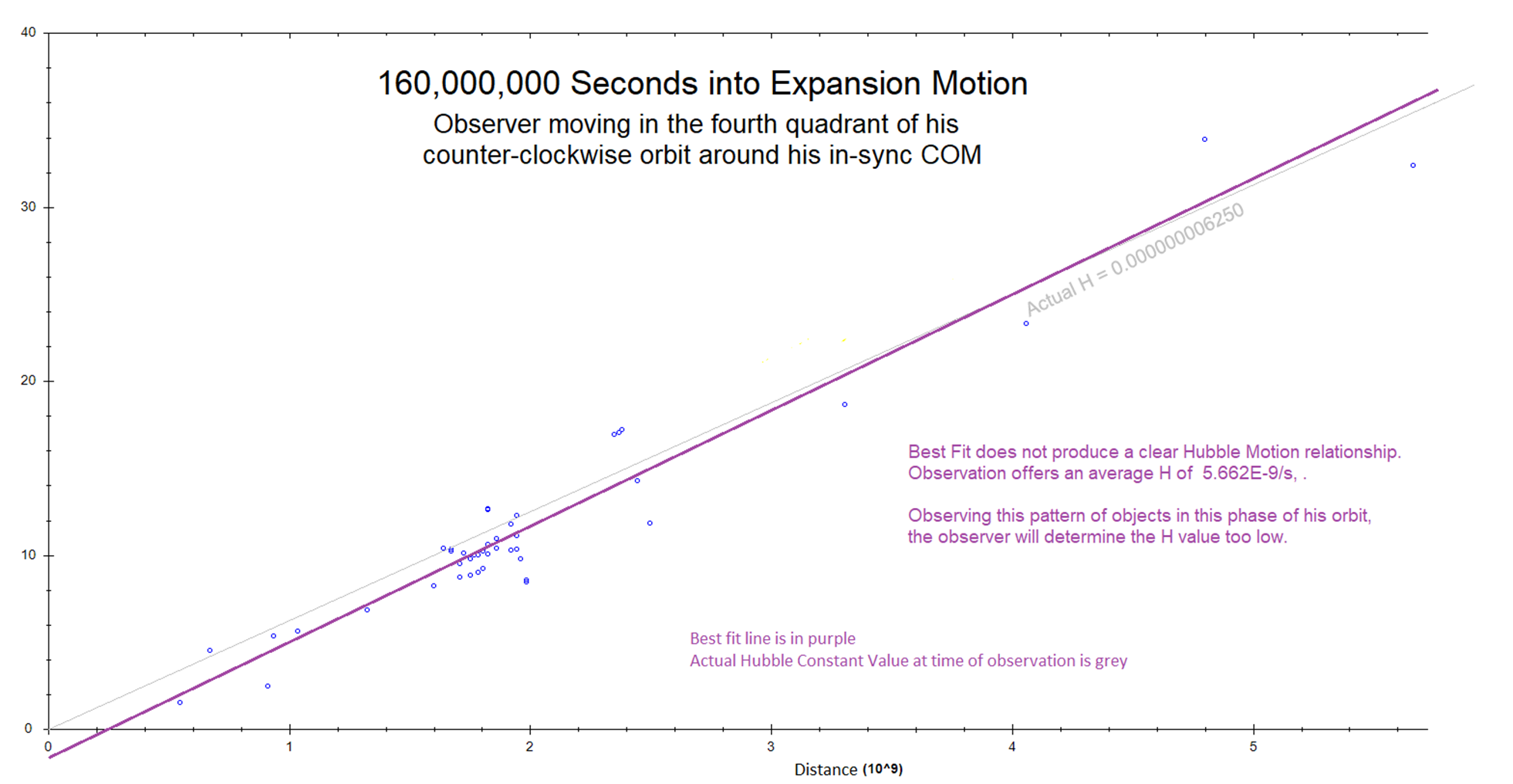
In this configuration of objects, uneven density around the
observer and his COM, none of the pauses to make observations yielded an
accurate Hubble Constant Value. The more lopsided the distribution around him
the more off the results and the direction of the errors for a given
configuration were influenced by what quadrant the observer was in.
Randomly
Generated “Homogeneuos” COM/Object Configuration, with Randomly Generated
Orbital Parameters
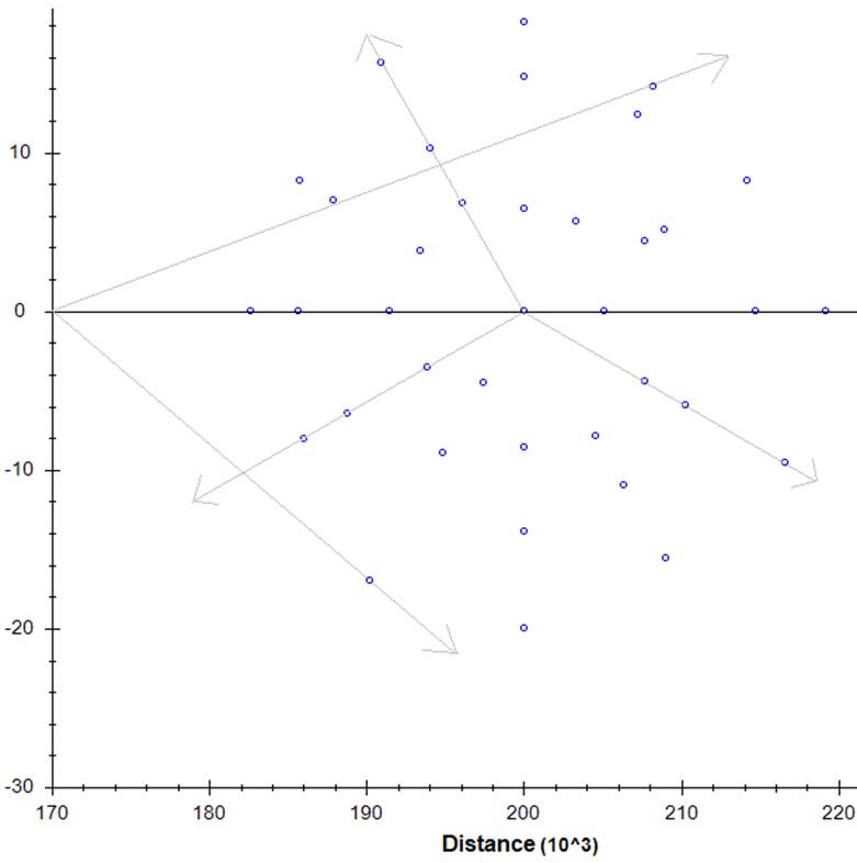
Adding orbits to COM’s in sync proved problematic to get an
accurate Hubble Constant Value, even from averages. The difficulty depended a
complicated mix of the configuration of the observer and the observation points
presenting him with data. I found that lopsided data (objects mostly in one
direction in his sky) presented the most difficulty for an observer to
calculate an accurate Hubble Constant Value. Not only is it difficult to cancel
out the skewing of results caused by the orbits by just adding many objects,
but the much easier task of canceling out skewing caused by the observer’s
orbit was not happening.
When the observer had an even distribution of objects around
him (for every object in one direction and distance there was an equal object
180 degrees) and all the orbits were in sync, then the percent error went down
to within a few percentage points. If I let the simulator randomly build the
orbits around the objects, it became problematic to get a reasonable estimate
of the Hubble Constant Value. Even with the skewing caused by the observer’s
orbits being averaged out, the orbits were causing chaos. Quantity of objects
helped, but strangely, as I let the simulator expand the disk, the accuracy
went up and down. It could range from 3% percent error to 25%. Distance
helped also, but when I let this simulator get very old it became flakey, it
seemed like the percent error was stabilizing into a range from 5 to 25%.
Even when the percent error was high, I could search through
the data to find two COM points that were 180 degrees apart around the
observer’s COM and the same distance away from the observer’s COM. If the
orbits where at least somewhat in-sync, I could then calculate a Hubble
Constant Value from the two objects and get an accurate estimate from their
average. This did not work if the objects selected were too much out of phase
in their orbits. If I instead found several object pairs in this configuration
the average was much more accurate, but the observer had no way to check the
results. From the observer’s perspective, it was always impossible to know if
current observations from even a carefully selected homogeneous configuration
was going to offer a good result. Sometimes it did, sometimes it didn’t. The
problem was not in the accuracy of the individual measurements but the
complexity of the interactions of orbits within the given configuration of
observation points.
Relative and
Observed Acceleration
I have not yet coded this new simulator to allow me to set
the COM’s out of sync. I suspect that if I do it will add the Relative
Acceleration or Deceleration in the closest objects. When the observer’s orbit
is throwing the observer away from center, he will observer a slight Relative
Acceleration in objects closest to him and that acceleration will decrease with
objects that are increasingly far away. If his orbit is throwing him back
toward center, he will see slight Relative Deceleration for objects closest to
him, likewise decreasing with distance away. All of my individual observation
points showed orbital acceleration and deceleration caused by the swinging of
the observer toward or away from his center by his orbit and the same for each
object. Relative Acceleration/Deceleration would be seen only in “local” or
close objects and it would fade away as distance increases. If I add COM out
of sync motion to this simulation, I suspect Relative Acceleration/Deceleration
will be a composite and more confusing.
Neither have I coded light delays into this new simulator,
which will be interesting because it will slow or increase the observed rates
of orbit for each object.
CMB verses
Observation: Observation questionable
If this Expansion Motion is current, it could suggest that
an observer will be unlikely to yield an accurate value of the Hubble Constant
Value from observations, especially if he thinks all the data points should
yield the same values. However, I could be that with extreme Expansion Age a
given configuration of distant objects would settle into a given range. If a
second configuration of objects is viewed at the same time that are within a
different range, say much closer, then the results could give a much lower or
higher value, depending on the lopsidedness and the observer’s orbit around his
COM. Closer objects would also be more susceptible to change by adding or
remove observation points.
More
Possible Real Observations Extracted from this Simulator
As I plotted these data charts, I recognized them. I posted
a chart, at the beginning of these simulations of orbital motions, made by Dr.
Hubble that looks like the plots that emerge from these new simulations.
The struggle to reconcile the Hubble Values from CMB verses Observation
be a struggle predicted by these simulations. I also just read that a new
value has come out of a study based on Red Giants. That value landed in
between the two old opposing values. This simulation would suggest that this
different set of data points, if grouped from a closer range or heavily clumped
arose a specific arc of the sky, could, and likely would, yield a significantly
different value.
The Age
of Expansion:
Without the disruptions in the pattern due to gravity and
light propagation (or even in those cases, at extreme distances), an observer is
able to use any expansion rate measured between two objects to determine how
long the disk has been expanding. Assuming that all points were once together
in one location at the beginning of the expansion, this would be the age of the
universe. The velocity observed between two objects divided by its velocity
will produce how long they have been diverging. The result should be the same
for every rate of expansion between two objects everywhere in the disk, so long
as the pattern is intact. Even if the
The speeds, or relative speeds, between the objects will
bring them back together in the same amount of time as all other objects. All
will come together back at center. In reality, during the time the two objects
are moving back together (he could be one of the two objects), he will not
realize that he will be returning to center himself. He would see the objects
moving directly toward him when they are actually both (or all) moving back
down their own axis toward center. His perceived reunion will be a mutual
return to center. In the time it takes them to unite, everything everywhere in
the disk will return to center with them. Objects badly skewed be gravity will
affect the accuracy.
An example from our data: Observer Y measured Object A at
166.67cm moving directly away from him at 3.33 cm/sec. That means it would
take that object 50.0 seconds to return to him at that speed. If motion were
reversed, he would see it coming directly toward him, but it is an illusion.
From the “actual” motion chart, at that same moment, Object A was moving
directly away from true center at 7.27cm/sec and was 360cm from center.
Observer Y was moving directly away from center at 5cm/sec and was 250cm from
center. It would take both of them 50 seconds to return to center, and this
would be their “actual” return motion.
Accelerating
Expansion verses Set Velocities
The motion in this model can be either an actual expansion
of the fabric of space or just mass drifting away from center under inertia. If
an actual expansion of space itself, then this simulation could also be done by
“pulling” each axis at an accelerated rate. If so, the data charts will show each
object accelerating away from center at a rate proportional to its distance
from center (see charts below – each axis is pulled at a rate of 5cm/s/s). At
each pause, the velocities of each object will still conform to the Hubble
formula, v = H * d, and all observations, illusions, and machanics will work
the same way. Therefore, in this model steady expansion or accelerated
expansion will both yield Hubble motion.
A difference will be in calculations of H. H = 1/t when
expansion was steady will no longer be valid:
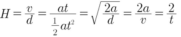
The H in an accelerating expansion will be double the value in
a steady rate expansion. Likewise, the age of the universe can no longer be
determined from dividing the distance observed by the corresponding velocity
observed. If the expansion is accelerating, you will have to determine the
observed acceleration and then decelerate the object toward closing the
observed gaps. This could help determine whether the expansion of the universe
is an acceleration or steady speed. If the age of the universe is known, either
the formula derived from steady rate expansion motion or the accelerated rate
motion should yield a reasonable estimate, but not both. If the universe
started out accelerating and then stopped, or started out steady and acceleration
started later, then neither formula would yield a reasonable approximation.
If this model is a steady speed expansion:
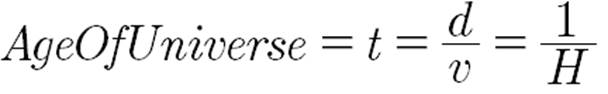
Convert current measurement of H units/sec:
AgeOfUniverse = 1/H = 1/2.333 X E-18/sec =4.28569XE17sec = 13,589,847,934
years
If this model is an accelerated expansion:
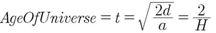
AgeOfUniverse = 2/H = 27,179,695,868 years
Actual and Observed motion for
Observer Y and Object A, if the expansion is an acceleration of 5cm/s/s
|
Time into expansion
|
Hubble
Value
|
Radius of Disk
after each expansion
|
Velocity of expansion
(outer most object)
|
Observer Y
new d
|
Velocity of
Y
|
Object A
R = 50
θ=60 deg
new y
|
Velocity of
A
|
Observed
Distance
|
Observed Velocity
|
Observed
θ
|
|
α
|
|
|
|
|
|
23.41
|
|
|
|
|
|
15 sec
|
0.133333
|
562.50
|
75
|
75.00
|
10
|
108.97
|
14.529
|
50.00
|
6.67
|
60
|
|
16 sec
|
0.125000
|
640.00
|
80
|
85.33
|
10.66
|
123.98
|
15.50
|
56.88
|
7.11
|
60
|
|
50 sec
|
0.040000
|
6250.00
|
250
|
833.33
|
33.33
|
1,210.78
|
31.96
|
555.49
|
22.22
|
60
|
|
51 sec
|
0.039216
|
6,502.50
|
255
|
867.00
|
34.00
|
1,259.69
|
48.91
|
577.93
|
22.67
|
60
|
|
5000 sec
|
0.000400
|
62,500,000.00
|
25,000.00
|
8,333,333.33
|
3,333.33
|
12,107,777.78
|
2,446.25
|
5,554,928.73
|
2,222.22
|
60
|
|
5001 sec
|
0.000400
|
62,525,002.50
|
25,005.00
|
8,336,667.00
|
3,334.00
|
12,112,621.37
|
4,843.59
|
5,557,150.92
|
2,222.67
|
60
|
|
Acceleration of each object due to expansion
|
|
|
5.00cm/s/s
|
|
0.667cm/s/s
|
|
0.9686cm/s/s
|
|
0.4444cm/s/s
|
|
Actual and Observed motion for
Observer Y and Object B, if the expansion is an acceleration of 5cm/s/s
|
Time into expansion
|
Hubble
Value
|
Radius of Disk
after each expansion
|
Velocity of expansion
(outer most object)
|
Observer Y
new d
|
Velocity of
Y
|
Object B
R = 50
θ=200 deg
new y
|
Velocity of
B
|
Observed
Distance
|
Observed Velocity
|
Observed
θ
|
|
α
|
|
|
|
|
|
-31.40
|
|
|
|
|
|
15 sec
|
0.133333
|
562.50
|
75
|
75.00
|
10.00
|
32.82
|
4.38
|
50.00
|
6.67
|
200
|
|
16 sec
|
0.125000
|
640.00
|
80
|
85.33
|
10.67
|
37.34
|
4.67
|
56.88
|
7.11
|
200
|
|
50 sec
|
0.040000
|
6250.00
|
250
|
833.33
|
33.33
|
364.67
|
14.59
|
555.61
|
22.22
|
200
|
|
51 sec
|
0.039216
|
6,502.50
|
255
|
867.00
|
34.00
|
379.40
|
14.88
|
578.06
|
22.67
|
200
|
|
5000 sec
|
0.000400
|
62,500,000.00
|
25,000
|
8,333,333.33
|
3,333.33
|
3,646,666.67
|
1,458.67
|
5,555,690.91
|
2,222.22
|
200
|
|
5001 sec
|
0.000400
|
62,525,002.50
|
25,005
|
8,336,667.00
|
3,334.00
|
3,648,125.48
|
1,458.96
|
5,558,823.70
|
2,222.67
|
200
|
|
Acceleration of each object due to expansion
|
|
|
5.00cm/s/s
|
|
0.667cm/s/s
|
0.2917cm/s/s
|
0.2917cm/s/s/
|
|
0.4444cm/s/s
|
|
Universal
Flash: CMB verses Observation
I read about a disparity between observation verses CMB in the
search for the current Hubble Constant value. It seemed to me that if the
light waves that make up the CMB are directionless, and all emitted at a common
moment (relatively speaking) in expansion, a “flash” in the Universe’s past,
then maybe I could use my simulator to play with something like that.
I wanted to use my simulator to create a universal flash with a
stationary observer to see through time. My observer would need to
receive an unlimited supply of light from increasingly far away distances in
all directions. Every second would bring new photons from objects that
were just a little further away than the object that emitted the light he just
measured.
I came up with a way to view this in my expansion simulator. I
could set my observer at center (which would render him expansion motionless)
and then every direction he looked would be α=0. Instead of placing billions of objects spaced evenly apart
along his line of sight, I could just use several objects and treat them as
samplings. I could then let the simulator expand the universe as it was
designed to do. I could then simulate a flash by extracting the data from
each object’s chart for a randomly selected moment for the flash. I could
place the extracted data (one row per object) in a new data chart as if was
data from one source, a composite object. The new chart would record the
emission position of each object at the time of the flash.
It occurred to me that the many flashes from many sources coming
from one direction would look to him like one continuous beam of light, as if
emitted from a single source. A continuous stream of photons from lined-up
sources could create the appearance of a single star in the sky receding from him.
It would be a “Phantom” object.
The composite chart would show how much time it takes for each
object’s light to reach the observer, how far away the emission point was, and
a offer a trace of the emission points observed and its virtual velocity.
I felt that information could be used to calculate a “Flash Hubble Value” using
the Hubble formula.
I had to alter the code that determines the length of time that
light travels between emitter and observer. Instead of knowing the observing position
and pushing the emitter back down its axis to know when the light he is seeing
was emitted (in the past), now the light emission point is frozen in place and
I had to know when its light will intercept the observer (in the future). Since
the observer is sitting still and the emission points frozen, the light bursts
will be the only movement.
In the sample data below, I selected 1000 seconds (HE=0.001) into the expansion as
the flash point.
In the first composite chart below
the observer is set at center, so not moving. I placed 5 objects on his
axis of motion, α = 0 and θ = 0, so all the objects are
lined up. Each row below is an extract from the individual object’s data
charts at 1000 seconds, the flash point for each of them. Since the location
of the flash points is frozen in time (all light observed in the future will
point back to them), the only thing moving is the emitted light, In the two
charts that follow it I set the observe moving slightly (using the out of sync
motion settings).
Data in chart below extracted from regular expansion data
charts. For each object data was selected from the 1,000 second point, HE=0.001:
Composite Chart 1 - Phantom
Object: Observer at center, not moving. Flash points are frozen in time: (no
expansion motion, the only motion is light), C=200cm/sec
|
|
Emitter
Distance from center
at time of flash
|
Observer distance from center at time of observation
|
Light Travel
Time
(since flash)
tf
|
Expansion
Time
at
Observation
|
Hubble
Value
at
Observation
|
Hubble
Value
of travel
Time
(Hf =
1/tf)
|
Phantom Object
Observed
Distance
Dr
|
Observed
Hubble
Constant
vr/Dr
|
Observed
θ
|
|
Obj 1
|
60,000.00
|
0
|
300
|
1,300.00
|
0.000769
|
0.003333
|
60,000.00
|
|
0
|
|
Obj 2
|
100,000.00
|
0
|
500
|
1,500.00
|
0.000667
|
0.002000
|
100,000.00
|
0.002000
|
0
|
|
Obj 3
|
200,000.00
|
0
|
1,000.00
|
2,000.00
|
0.000500
|
0.001000
|
200,000.00
|
0.001000
|
0
|
|
Obj 4
|
400,000.00
|
0
|
2,000.00
|
3,000.00
|
0.000333
|
0.000500
|
400,000.00
|
0.000500
|
0
|
|
Obj 5
|
1,000,000.00
|
0
|
5,000.00
|
6,000.00
|
0.000167
|
0.000200
|
1,000,000.00
|
0.000200
|
0
|
|
|
940,000cm
vP=200cm/s
|
0
vO=0cm/s
|
4,700 sec
|
4,700 sec
|
|
|
940,000cm
vr=200cm/s
|
|
|
Vr =  = C
= C
Composite Chart 2 - Phantom
Object: Observer at center, moving at 10cm/sec. Flash points are frozen in
time, C=200cm/sec
|
|
Emitter
Distance from center
at time of flash
|
Observer distance from center at time of observation
|
Light Travel
Time
(since flash)
tf
|
Expansion
Time
at
Observation
|
Hubble
Value
at
Observation
|
Hubble
Value
of travel
Time
(Hf =
1/tf)
|
Phantom Object
Observed
Distance
Dr
|
Observed
Hubble
Constant
vr/Dr
|
Observed
θ
|
|
Obj 1
|
60,000.00
|
11,428.57
|
242.8571
|
1,242.86
|
0.000805
|
0.004118
|
48,571.43
|
|
0
|
|
Obj 2
|
100,000.00
|
13,333.33
|
433.3333
|
1,433.33
|
0.000698
|
0.002308
|
86,666.67
|
0.002308
|
0
|
|
Obj 3
|
200,000.00
|
18,095.24
|
909.5238
|
1,909.52
|
0.000524
|
0.001099
|
181,904.76
|
0.001099
|
0
|
|
Obj 4
|
400,000.00
|
27,619.05
|
1,861.90
|
2,861.90
|
0.000350
|
0.000537
|
372,380.95
|
0.000537
|
0
|
|
Obj 5
|
1,000,000.00
|
56,190.48
|
4,719.05
|
5,719.05
|
0.000175
|
0.000212
|
943,809.52
|
0.000212
|
0
|
|
|
940,000cm
vP=210cm/s
|
44,761.9
vO=10cm/s 1
|
4,476 sec
|
4,476.19 sec
|
|
|
895,238cm
vr=200cm/s
|
|
|
Composite Chart 3 - Phantom
Object: Observer at center, moving at -10cm/sec. Flash points are frozen in
time, C=200cm/sec
|
|
Emitter
Distance from center
at time of flash
|
Observer distance from center at time of observation
|
Light Travel
Time
(since flash)
tf
|
Expansion
Time
at
Observation
|
Hubble
Value
at
Observation
|
Hubble
Value
of travel
Time
(Hf =
1/tf)
|
Phantom Object
Observed
Distance
Dr
|
Observed
Hubble
Constant
vr/Dr
|
Observed
θ
|
|
Obj 1
|
60,000.00
|
-12,631.58
|
363.1579
|
1,363.16
|
0.000734
|
0.002756
|
72,631.58
|
|
0
|
|
Obj 2
|
100,000.00
|
-14,736.84
|
573.6842
|
1,573.68
|
0.000635
|
0.001743
|
114,736.84
|
0.001743
|
0
|
|
Obj 3
|
200,000.00
|
-20,000.00
|
1,100.00
|
2,100.00
|
0.000476
|
0.000909
|
220,000.00
|
0.000909
|
0
|
|
Obj 4
|
400,000.00
|
-30,526.32
|
2,152.63
|
3,152.63
|
0.000317
|
0.000465
|
430,526.32
|
0.000465
|
0
|
|
Obj 5
|
1,000,000.00
|
-62,105.26
|
5,310.53
|
6,310.53
|
0.000158
|
0.000188
|
1,062,105.26
|
0.000188
|
0
|
|
|
940,000cm
vP=190cm/s
|
-49,473.68
vO= -10cm/s
|
4,947.37 sec
|
4,947.37 sec
|
|
|
989,473cm
vr=200cm/s
|
|
|
·
The observer
sees every Phantom Object moving directly away from him at the speed of light, whether
he is sitting still or moving.
·
There is
a Flash Hubble Constant Value Hf = 1/tf , where tf = Age of flash.
·
Every
“flash” has an independent Hubble Expansion, its own Hubble Constant Values.
·
Since the
relationship of the Phantom Object and the observer is Hubble Motion, Hf is reducing with time.
·
With age,
Hf becomes more and more of a constant, depending on sensitivity of
data.
·
If the
observer is set in motion, looking in the direction of motion, the perceived
density of the emission points will increase and the time to view them will
decrease.
·
If the
observer is set in motion, looking in the opposite direction of motion, the
perceived density of the emission points will decrease and the time to view
them will increase.
The observation of receding objects and the observation of the
remnants of a flash both present Hubble Motion relationships that are
independent of each other:

Chart 1 is an observer siting still and observing the light from
the flash as it reaches him. In Charts 2 & 3, the observer is in motion.
I used my formula for a conversion constant that I derived from light
propagation delays to try to express the compression rates in the bottom rows
of the charts. The distances are not to real objects but to light burst
points. It is more like a frequency of light bursts being viewed:
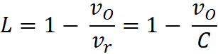
where vO=velocity
of observer, and C is the speed of light (vr=C).
It seemed to almost work. This formula was off by a consistent
factor unique to each chart for all my simulations of phantom objects with my
observer in motion. By trial and error (so not sure why this works) I found a
formula that expresses the factor I needed for each chart to make my old
formula work. I used it to come up with a conversion formula for phantom objects
in motion, as viewed by an observer not in motion, to motion observed for the
same phantom object while he is in motion. I called the conversion factor LP:
The correction factor is the
reciprocal of 
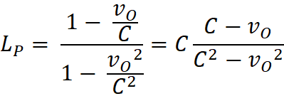
From this conversion factor I could translate observations of
compression of time and distance (totals in the bottom rows) from my observer
not in motion to my observer in motion:


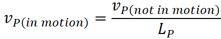
From Chart 2 (Observations of
the flash in the direction the observer is moving; C = 200, vO = 10)
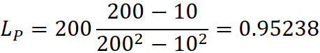

From Chart 3 (Observations of
the flash in the opposite direction the observer is moving; C = 200, vO
= -10)
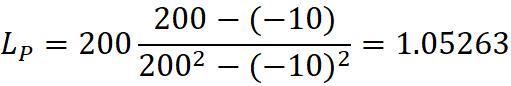
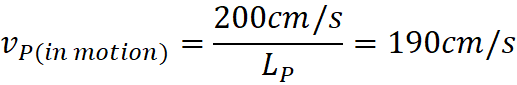
For every scenario, observed light
bursts present the observer with a Phantom object moving away from him at the
speed of light (vr). When the observer is in motion the flux of
emission points changes, observed frequencies increase or decrease (vP).
New Simulator: Flash motion
My Expansion simulator
couldn’t examine a flash at various angles, so I coded a new simulator to focus
on flash events. To do that, I worked backwards from the observation to the
virtual motion of the Phantom object (which again is not a physical object but
a trace of the emission points that provide the light of observation, as if it
was a single object doing the emitting. The trace would provide the rate, or
frequency, that emission points are viewed.) I built into this new simulator the
ability of the observer to watch at various angles.
I built the new simulator to
conform the observer to the expansion pattern of the previous simulator,
(v=distance from center/age of expansion, moving directly away from expansion
center). As I ran more and more simulations, I began to see that this was not
necessary because the observation of a flash turned out to be completely
dependent on the motion of the observer, in sync or not, and independent of
the ongoing expansion round him.
Step one of my new simulator
was to determine the distance from the observer’s current position to the
emission point of the current pulse of light being viewed;
Observed
distance = (Age of Flash) * C
From that physical distance, I
calculated the physical location based on the angle he is looking. From that,
the distance to the center of expansion and the divergent angle α.
This was how my simulator
worked. I began running simulations and plotted the results. On my first plot I
could see that the emission points were forming a straight line. I could see
immediately that α was changing with time.
Yet, when I drew a line through them the trace it created was a straight line.
The line did not pass through expansion center. It traced a virtual path that intersected
the real path of the observer at his position, where he was, when the flash
happened.
The data and plots resembled
the suggestions from my expansion simulator, that the Flash has its own
expansion motion relationships, its own Hubble Motion Values, and now I could
clearly see them starting at the moment of the flash. I then added a
calculation of α at the “Flash Point” along
the observer’s path and reran the simulations. This new α did not change with time.
There was Hubble Motion between the observer and the Phantom Object, both would
have left a common point at a set velocity.
The virtual velocities of some
of the phantom objects exceeded the speed of light and some didn’t. Since these
are not real objects, but frequencies of emission points, this was not a
violation. The paths aren’t a velocity but represent the distribution of
emission points observed at the angle of observation. The virtual path was providing
the rate, or flux, at which the observer was seeing light pulses go past him.
The relative velocity of the “observed” phantom objects, no matter how many
pulses per second were representing them, is always the speed of light, but the
trace of the emission points creating it might be above or below it. When I
plotted full simulations I saw how important this was, a boundary appeared
between red and blue shift observations.
Plot of a simulation with
observer at center, not moving.
The speed of light in this
simulation is 200cm/s. Therefore, this plot represents the base (at rest)
frequency of observed pulses, which turns out to always be C * density of
emitters at the time of the flash.
Observer
velocity: 0cm/s
Θ = varying degrees (all look
the same to the observer when he is not moving)
Flash point:
1000 seconds into expansion
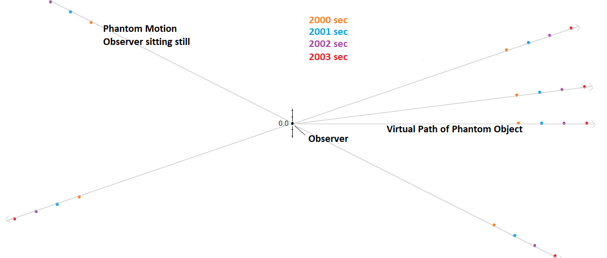
Data Chart of Observer not Moving
Observer
velocity: 0cm/s
Θ = 0 degrees
Flash point:
1000 seconds into expansion
C=200cm/s
|
Age
of
Expansion
|
α
at
center of expansion
|
Observer
Distance
From
Expansion
Center
|
Emission
Point
Distance
from
Center
|
α
at
flash point
(Position
of Observer at time of flash)
|
Emission
Point
Distance
from
Flash
Point
df
|
Time
For
Light
to reach
Observer
tf
|
Observed
Distance
Dr
|
Calculated
Hp
(vr
/Dr)
(1/
tf)
|
|
2000
|
0
|
0.00
|
200,000.00
|
0
|
200,000.00
|
1,000.00
|
200,000.00
|
0.0010000
|
|
2100
|
0
|
0.00
|
220,000.00
|
0
|
220,000.00
|
1,100.00
|
220,000.00
|
0.0009090
|
|
2200
|
0
|
0.00
|
240,000.00
|
0
|
240,000.00
|
1,200.00
|
240,000.00
|
0.0008333
|
|
2300
|
0
|
0.00
|
260,000.00
|
0
|
260,000.00
|
1,300.00
|
260,000.00
|
0.0007692
|
|
|
|
DO=0cm
vO=0cm/s
|
|
|
Df=60,000cm
vP=200.00cm/s
|
|
Dr=60,000cm
vr =200cm/s
|
|
If there were 3 per cm emitters at the moment of the flash then
the observer is seeing: vp * 3 = 600.00 pulses per second (at rest
frequency)
Data Chart of Observer Moving
at 10cm/s and looking 30 degrees from his forward motion axis:
Observer velocity:
10cm/s
Θ = 30 degrees
Flash point:
1000 seconds into expansion
C=200cm/s
|
Age
of
Expansion
|
α
at
center of expansion
|
Observer
Distance
From
Expansion
Center
|
Emission
Point
Distance
from
Center
|
α
at
flash point
(Position
of Observer at time of flash)
|
Emission
Point
Distance
from
Flash
Point
|
Time
For
Light
to reach
Observer
tf
|
Observed
Distance
Dr
|
Calculated
Hp
(vr
/Dr)
(1/
tf)
|
|
2000
|
27.37
|
20,000.00
|
217,550.46
|
28.62
|
208,720.15
|
1,000.00
|
200,000.00
|
0.0010000
|
|
2100
|
27.48
|
21,000.00
|
238,417.86
|
28.62
|
229,592.17
|
1,100.00
|
220,000.00
|
0.0009090
|
|
2200
|
27.57
|
22,000.00
|
259,286.00
|
28.62
|
250,464.18
|
1,200.00
|
240,000.00
|
0.0008333
|
|
2300
|
27.65
|
23,000.00
|
280,154.71
|
28.62
|
271,336.20
|
1,300.00
|
260,000.00
|
0.0007692
|
|
|
|
DO=3,000cm
vO=10cm/s
|
|
|
Df=
62,616.05cm
vP=208.72cm/s
|
|
Dr=60,000cm
vr =200cm/s
|
|
If there were 3 per cm emitters at the moment of the flash then
the observer is seeing: vp * 3 = 626.16 pulses per second
Plot of the
above chart
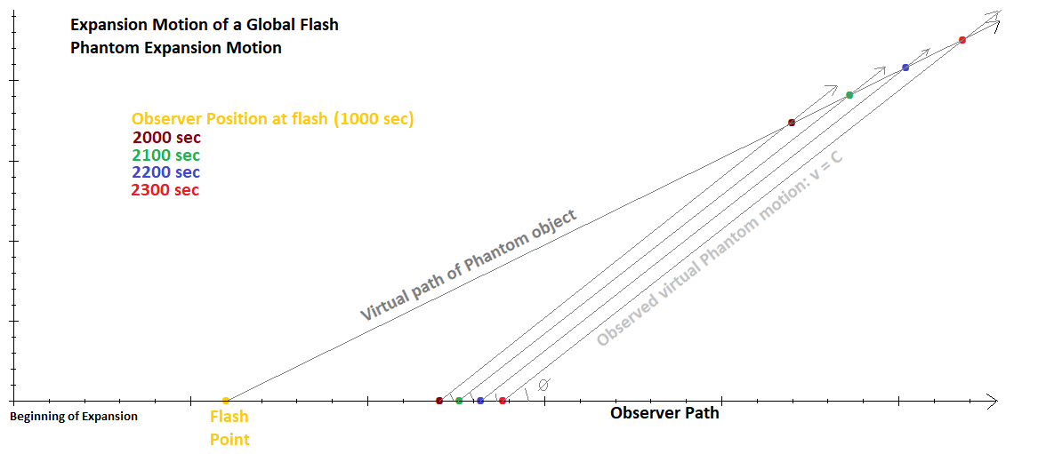
Plot of the
same data but from the observer’s perspective (observed or relative motion)
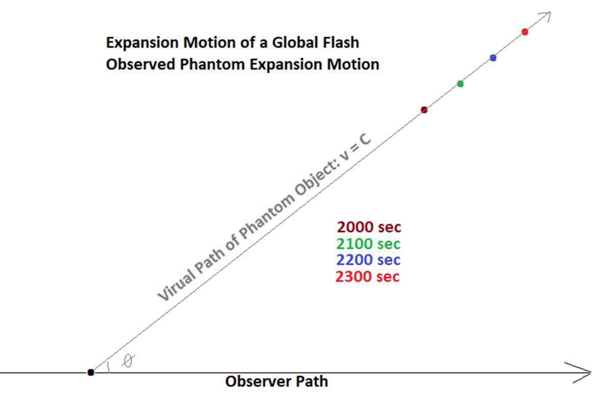
Data Chart of Observer
looking 170 degrees from forward motion axis:
Observer
velocity: 10cm/s
Θ = 170 degrees
Flash point:
1000 seconds into expansion
C=200cm/s
|
Age
of
Expansion
|
α
at
center of expansion
|
Observer
Distance
From
Expansion
Center
|
Emission
Point
Distance
from
Center
|
α
at
flash point
(Position
of Observer at time of flash)
|
Emission
Point
Distance
from
Flash
Point
|
Time
For
Light
to reach
Observer
tf
|
Observed
Distance
Dr
|
Calculated
Hp
(vr
/Dr)
(1/
tf)
|
|
2000
|
168.90
|
20,000.00
|
180,337.29
|
169.48
|
190,159.85
|
1,000.00
|
200,000.00
|
0.0010000
|
|
2100
|
168.95
|
21,000.00
|
199,352.39
|
169.48
|
209,175.84
|
1,100.00
|
220,000.00
|
0.0009090
|
|
2200
|
169.00
|
22,000.00
|
218,367.65
|
169.48
|
228,191.82
|
1,200.00
|
240,000.00
|
0.0008333
|
|
2300
|
169.04
|
23,000.00
|
237,383.02
|
169.48
|
247,207.81
|
1,300.00
|
260,000.00
|
0.0007692
|
|
|
|
DO=3,000cm
vO=10cm/s
|
s
|
|
Df=
57,047.96cm
vp=190.16cm/s
|
|
Dr=60,000cm
vr =200cm/s
|
|
If there were 3 emitters per cm at the moment of the flash then
the observer is seeing: vp * 3 = 570.48 pulses per second
Plot of Relative Motion from above chart
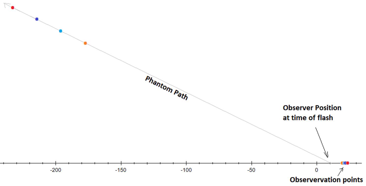
Observer looking directly behind him.
Observer
velocity: 10cm/s
Θ = 180 degrees
Flash point:
1000 seconds into expansion
C=200cm/s
|
Age
of
Expansion
|
α
at
center of expansion
|
Observer
Distance
From
Expansion
Center
|
Emission
Point
Distance
from
Center
|
α
at
flash point
(Position
of Observer at time of flash)
|
Emission
Point
Distance
from
Flash
Point
df
|
Time
For
Light
to reach
Observer
tf
|
Observed
Distance
Dr
|
Calculated
Hp
(vr
/Dr)
(1/
tf)
|
|
2000
|
0
|
20,000.00
|
180,000.00
|
0
|
190,000.00
|
1,000.00
|
200,000.00
|
0.0010000
|
|
2100
|
0
|
21,000.00
|
199,000.00
|
0
|
209,000.00
|
1,100.00
|
220,000.00
|
0.0009090
|
|
2200
|
0
|
22,000.00
|
218,000.00
|
0
|
228,000.00
|
1,200.00
|
240,000.00
|
0.0008333
|
|
2300
|
0
|
23,000.00
|
237,000.00
|
0
|
247,000.00
|
1,300.00
|
260,000.00
|
0.0007692
|
|
|
|
vO=10cm/s
|
|
|
Df=57,000.00cm
vp=190.00cm/s
|
|
Dr=60,000cm
vr =200cm/s
|
|
If there were 3 emitters per cm emitters at the moment of the
flash then the observer is seeing: vp * 3 = 570.00 pulses per second
(It turns out that the observer’s position at flash is also
virtual, not necessarily on his axis away from expansion center. With this Flash
analysis, his current axis of motion points back to a projected position where
he would have been at time of flash based on his current velocity. He may
never have actually been in that position. In this analysis, if he changes
direction his “projected location at the moment of the flash” instantly moves
with him.)
The data from my first simulator used to evaluate observation of a
past universal flash was from the perspective of watching a common set of flash
points with my observer at different speeds. To compare this Flash Simulator’s
data to that data the same span of emission points needs to be watched. Since that
was not the way this simulator works, I had to calculate it:

Using the data chart for the observer moving at 10cm/s and
watching at 30 degrees:
I had to reevaluate the conversion factor formula derived from the
Flash analysis in the Expansion simulator to take into account different angles
of observation:
From the equations derived using
the first simulator:


The two simulators are producing the same relationship of
motions. The Expansion Simulator could only watch a set of emission points
from different observational perspectives. The Flash Simulator gives a
perspective of observations from light emitted at set moments in time for the
observer. It also allows for evaluations of movement relationships at any
direction desired.
Determining the speed of the trace
(vpt)
(the virtual velocity of the Phantom object)

vp = speed of Phantom object (or trace of emission
objects through space)
vo = speed of observer
θ = angle observer is watching against his forward motion
t = time since flash
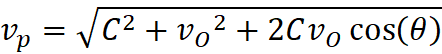
Vector Analysis:
Since the motion of the observer and the relationships with the
Phantom object create Hubble Motion, I can explore a flash using relationships
from “Source of the Illusions”.
Since in “prefect” Hubble Motion the horizontal vectors cancel out
only the observed (relative) perpendicular velocity vectors are needed to
evaluate Phantom object motion:

Since the observed (relative) velocity (vr ) for a phantom object is
always C:
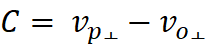
The velocity of the Phantom object (vp) is going to be
greater than light speed and can be calculated:


Therefore, I should be able to determine α (the angle between the
observer and his emission points path at the projected position where the
observer was be at the point of flash):
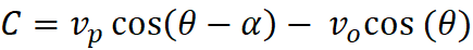
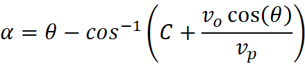
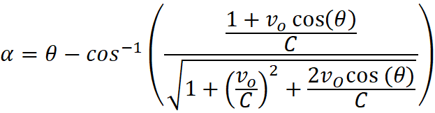
Phantom objects are not real objects, but represent flash points observed
since the flash, a frequency of light bursts in objects/cm.
If ρf is the density of emitting objects at the time of the flesh
(emission points/cm) then the frequency of observed emission points is,
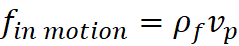
The frequency observed of the flash when the observer is at rest
(vO=0) is measured when the observer is not moving, that is when he
is located at the center of expansion. When the observer is at rest the
velocity of the phantom objects in every direction will be C (that is, the
trace will be moving across the sky at C).
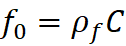
Therefore:
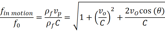
Using the vector relationships this can also be expressed as
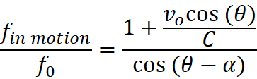
Plot of full simulation: Observer’s Perspective at rest (located
at true expansion center)
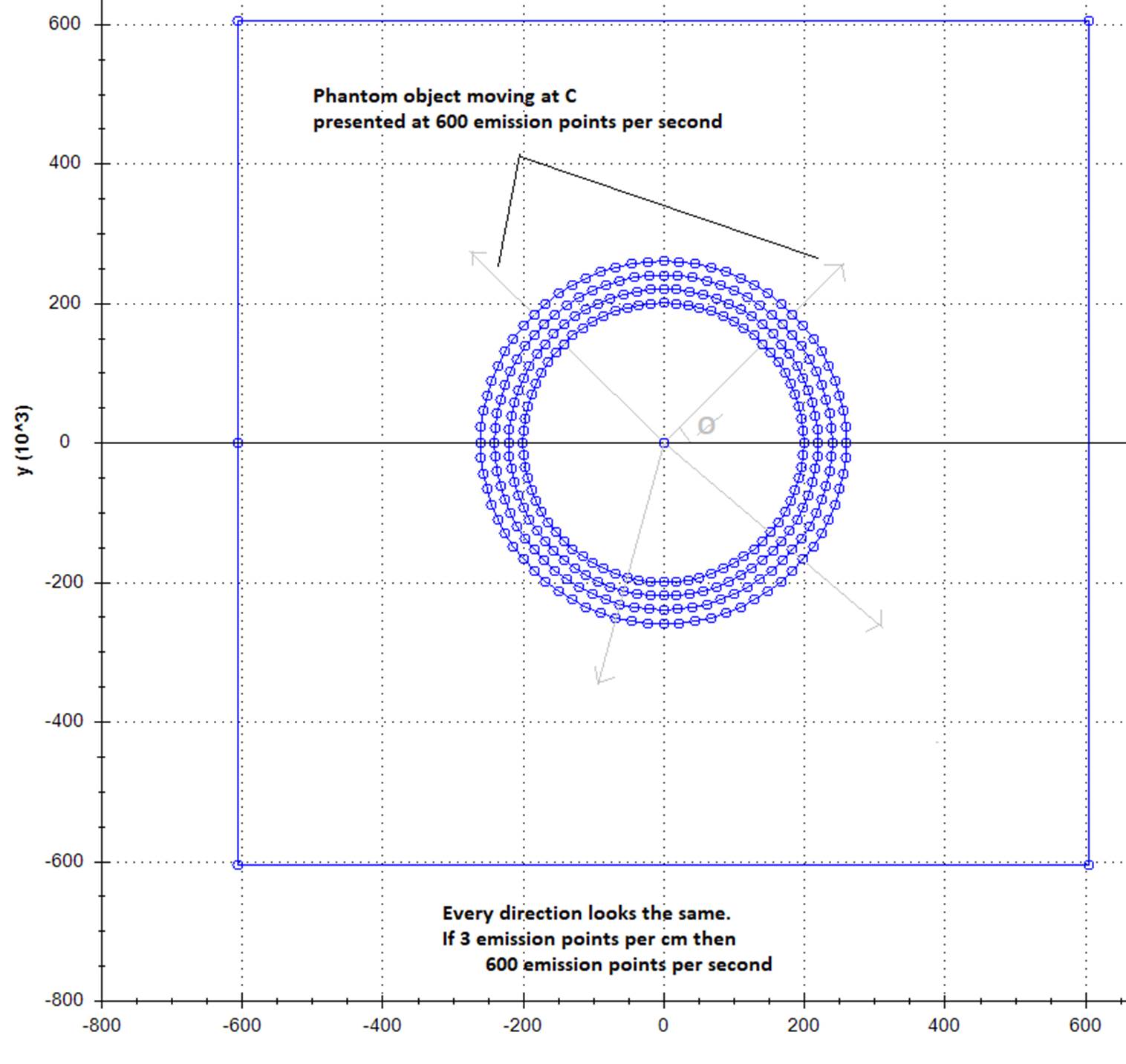
Plot of full simulation: Observer in motion (velocity = 75% of
light speed):
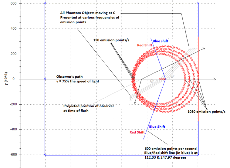
Plot of full simulation: Observer in motion (velocity = 5% of
light speed):
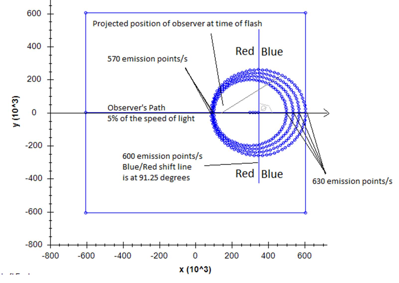
Reducing the speed of the
observer alters the frequencies shift of observed emission points, and the
angles of the Red/Blue shift transition boundaries. Only the speed of light
alters the base frequency rate at which that boundary is defined.
I ran many simulations using
various speeds for light. The plots above are samples using 200cm/sec. I used
values as high as 300,000cm/s. The higher the speed of light the higher the frequency
values observed for emission points at any angle. No matter what value I used there
was a boundary (an angle) between Red and Blue Shift observations that was defined
by the speed of light. That was true because the Red/Blue Shift Boundary was
demarcated by the frequency of observed mission points with observer at rest,
which is C *density of the universe at the time of the flash. The upper
boundary, when my observer’s speed was approaching the speed of light was 120
degrees, regardless of the speed light I used. The lower boundary was when he
was approaching 0 speed. Each speed of light has its own unique at rest
frequency that defines this boundary.
The angle of the Blue/Red Boundary
depends on the observer’s motion and appears to be a factor of his speed as a
percentage of the speed of light.


This Red/Blue Shift Doppler
boundary for any flash is demarcated by the angle at which the virtual velocity
of the trace path (vp) is equal to the observed (relative) velocity
of the Phantom object which is always C,( vP = vr = C). vP
and vr are equal when the observer is at rest. Therefore, at this
angle, the observed frequency of pulses equals the frequency observed when the
observer is at rest.
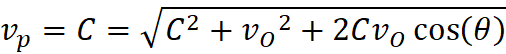
Therefore,

There are two points around a circle
that will yield this value of cos. The other is,

This could be the first hope
of the observer determining his velocity in the universe. If he can get a
frequency reading of the flash all the way around him and find the Angle of
Red/Blue Shift, he can determine his velocity, but still no way to orient
himself toward center. (Not knowing the nature of his out-of-sync situation.)
In the “Plot of Full
Simulation” the simulation discovered the boundary to be at 112.03 degrees. From
this observation, the observer can calculate his speed in the universe, but it
tells him nothing about his direction:
vo = - 2C cos(“Angle of Red/Blue Shift Boundary”) = - 2C cos(112.03)
= 150.04cm/s
The actual velocity I set for the observer was 150cm/s (75% the
speed of light).
Both simulators suggest that
the Hubble Constant value for a flash, Hf, is not the same as that of
the observational expansion, HE. In this simulator, HE – Hf, will give the observer the
time in history of the flash. That implies that if HE < Hf, , the flash happened before physical
expansion began. That doesn’t play well with current theories.
Even so, I am including this idea -- for one, because I have been
including whatever comes out of my simulator even when it seemed that actual
observations would invalidate it (only to then learn that it doesn’t). I
decided to include it also because I wonder now if light propagation from a flash
event, with emission points frozen in place, just might not ever offer the same
Hubble Constant Value as an ongoing expansion motion of light emitting objects.
Unless the flash and the expansion are simultaneous, they do not make the same
presentation. Observation of a flash is always a straight line
between the point of emission and the point of observation. Moving
emitting objects dictate location of the emission points that make up the
continuous beam of light. A flash can substitute emission points to
maintain motion of a phantom object, keeping it always directly away from the
observer, wherever he looks. A flash presentation doesn’t care what
generated the light.
Current theory about space itself expanding might demand that the
red shift of received light comes from the expansion of the space it is
traveling through. If that theory requires the two offer the same value, but
they don’t, it might mean that stretching space is not what is stretching
wavelengths.
When the
flash happened: Density of the Universe
There may be a way the observer can determine the time,
within the expansion, that the flash occurred (that is, if the flash is a part
of the expansion). In the expansion pattern of the first simulator, if the
density of all mass starts out homogeneous then it will remain so throughout
expansion, from the center of the expansion to the outer reaches, density will
decrease evenly with time. If the light was emitted from mass caught up in the
expansion, then it contains information about the physical density of the
Universe at the time of the flash (emission points per cm). If that is
discernable, and if he can determine the current physical density, then an
observer can use that link between the two determine when the flash happened.
In this simulation, to determine the density of his universe
in the present, the observer can measure the distance (dR) to a far-off object
(where measurable Hubble motion is linear -- out beyond relative acceleration
and dark flow) and count the number of objects between him and it.
 =
=
where vR is relative velocity
of the observed object
Since this is Hubble relationships, the object count between
the observer and his distant object is constant so he can use his count and Hubble
Motion parameters of the outer object to determine the density of the universe
at any time in history,
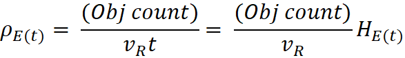
where t is the historical time
desired and HE
is the current Hubble Constant Value from observation.
The flash point positions are frozen in time and each flash
point represents the position of the emitter (object) at the time of flash. The
emission points he is observing contain a record of the density of the Universe
at the time of the flash.

where vP
is the speed of the trace of observed emission points.
Δt is the timespan that emission points are
counted.
If he measures his emission points while looking at the
angle of red/blue boundary, then vP=C,
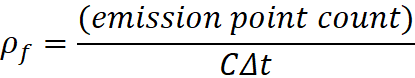
This simulator offers a way to determine the density of
universe at the time of the flash (ρf) from observable parameters:
The observer can measure the
emission point frequency of the flash at 0 and 180 degrees.
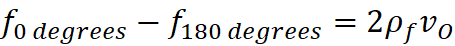
Also, at θ = 90 degrees,
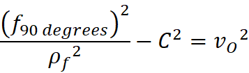
Solve both for vo and setting them
equal, he can solve for the density at the time of the flash in terms of
strictly observable data:
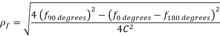
He can also determine his own
velocity in the universe from strictly observable data
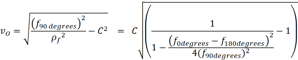
If he knows his velocity…
he can determination the density
of the universe at the time of the Flash using a single reading taken at the
Red/Blue shift Boundary:

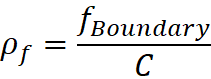
Or from
a reading made at ANY angle
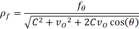
Knowing the density of the universe at the time of the
flash, he can determine when the flash happened. The flash would have happened
when the density of the universe was the same as the density recorded within
the flash,
 where t is the time of the flash

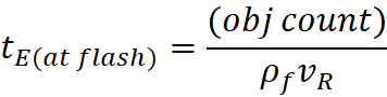
Therefore, the density of the Universe can be used to
determine the expansion Hubble Constant Value at the time of the flash:
HE(at flash) = 1/tE(at flash)
In the simulation that generated Chart 3 I set the density
at the time of flash at 3 objects per cm. I set the time of the flash to be
1,000 seconds into expansion. So, if my observer watches at his red/blue shift
angle for 5 seconds he will count 3,000 emission points (objects). He would
then calculate the density of the Universe at the time of the flash:
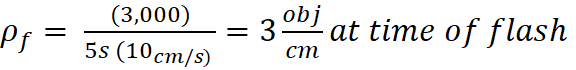
He can confirm this using direct observation data (the
values below extracted from data used to create Chart 3):
f0degrees
= 630.0000 e/s (observed emission points/s at time of observation which
represent objects/s viewed at time of flash)
f90degrees
= 600.7495 e /s
f180degrees
= 570.0000 e /s
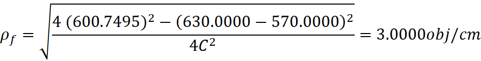
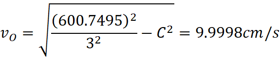
Knowing the density observed in the flash, the time of the
flash can be calculated. Chart 3 started at 2,000 seconds into expansion. If
my observer spots an object 10,000cm away (and it is in sync) he will measure
its relative velocity to be 5cm/second (vE =HdE, where H=0.0005). He would count 15,000 objects
between it and him.

This calculation is not the time since the flash, from which
the Hubble Constant for the flash could be determined. This is the expansion
time at the time of the flash. I want to know the H of the flash verses the H
of expansion.
The “Flash Hubble Constant Value” at time of observation can
be directly measured from current observations of the flash combined with current
observations of the universe. If the observer selects a distant object moving
away from him in clean Hubble motion:

ð 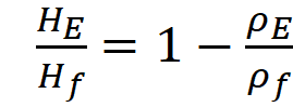
where
HE
= Current Expansion Hubble Constant Value
Hf
= Current Flash Hubble Constant Value
vR
= the relative velocity of the observed object
d = distance to observed object
#objs = number of objects between the observer and the
observed object
ρE
= Current density of the universe (#objs/d)
ρf
= Density of the universe at the time of the flash
The Flash Hubble Value can be calculated from current
measurable flash and expansion parameters:
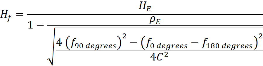
where
f is the emission points counted
in the observed light from the flash
What’s
true in this disk is true in a sphere:
Since our disk was sliced from a sphere such that the
center, the observer, and the observed object define the slice, and since you
could therefore rotate this disk within the sphere in any direction or
orientation, all observations remain true anywhere within the sphere.
Homogeneous
Expansion:
If you place evenly distributed dots on a rubber band and
stretch it, the space between each dot increase at the same rate, proportional
to the length of the band. The density drops with time, inversely proportional
to the length of the band. Current observations offer that space is homogeneous,
if that were not so this model would be ruled out.
Example:
If we look at two circles of
observation around the observer and make the distribution of objects around
each to start out with the same density, how will the densities compare as
Expansion Motion progresses?
At 10,000 seconds into Expansion
Motion
First Circle: R = 1,000cm from
center (or the Observer).
Therefore, rate of expansion away from center (or observer):
.1cm/s.
Circumference of circle: 6,283cm
Number of objects on circle: 628
Arch distance between objects: 10cm (approx.)
Density: 0.1 objects/cm
Second Circle: R = 5,000cm from
center (Observer)
Rate of expansion away from center (or observer): .5cm/s.
Circumference of circle: 31,416cm
Number of objects on circle: 3,142
Arch distance between objects: 10cm (approx.)
Density: 0.1 objects/cm
At 50,000 seconds into Expansion
Motion
First Circle: R = 5,000cm from
center (or Observer).
Rate of expansion away from center (or observer): .1cm/s.
Circumference of circle: 31,416cm
Number of objects on circle: 628
Arch distance between objects: 50cm (approx.)
Density: 0.02 objects/cm
Second Circle: R = 25,000cm from
center (or Observer)
Rate of expansion away from center (or observer): .5cm/s.
Circumference of circle: 157,080cm
Number of objects on circle: 3,142
Arch distance between objects: 50cm (approx.)
Density: 0.02 objects/cm
If the event that gave mass this motion also distributed
mass evenly (homogeneously), then every unit of mass would experience every
other moving away at the same rates. If truly homogeneous, the net force of
gravity on each unit of mass would be net zero (perhaps even at the atomic
force level). From the center of the sphere, where everything is moving the
slowest, until you approach the outer edges, density would drop with time, but
remain the same everywhere. (It would seem reasonable that as you approach the
outer most fringes mass would feel a pull back toward center.)
Even once disrupted, the merged masses and Centers of
Momentum will reflect the original distribution at the start of Expansion
Motion, and this pattern of motion.
Luminosity
and Acceleration
Just a
thought: When reading about “Dark Flow” in one article a scientist wrote that
under Hubble Motion theory holds that there should never be lateral motion caused
by Expansion. I also read that the reason Dr. Adam Weiss declared the
Expansion of our Universe to be accelerating is because very distant galaxies
appear dimmer than they should be at their calculated distance due to Hubble
Motion. I assume that under current Expansion Theory the angle of Expansion
motion between two objects will always be zero. I found a basic General
Relativity equation for luminosity (I think).
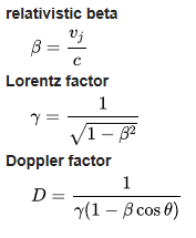
Using
this equation, relativistic beta’s influence on the apparent brightness of a
star would be minimum for Expansion motions under current Expansion Theory
(since cos θ = 1). Therefore, under current Expansion Motion theory General
Relativity would dim luminosity at a minimum.
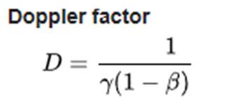
However,
in the pattern of my simulator θ would rarely be zero (see image below). In
my simulations, θ spans the range of 0 to 90 degrees. Every observed
object is much more likely to have a value > 0 and less than 90.
Therefore, if General Relativity were applied to the pattern of Expansion in my
simulator, virtually every far distant object (with relative velocities
approaching large values) would be expected to exhibit a lowered luminosity,
which Dr. Weiss reports is observed and under current Expansion Theory, would
require our Universe to be under an accelerating Expansion. Or, combined with
not being able to detect Dark Energy, it could be a clue that the current
theory is not right.
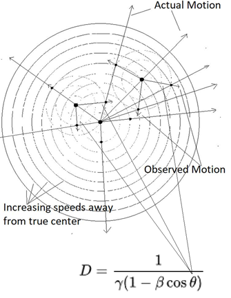
This model
would not have to be an ongoing expansion force:
If objects are moving away from each other due to the fabric
of space expanding, that suggests an interface, or friction, between space and
mass. If so, how is it that we observe mass traveling frictionless through
space? If there is friction when space moves past mass, then there is friction
when mass moves through space.
This pattern suggests a way that the universe would not have
to be an ongoing expansion of space itself for every observer to perceive
himself located at center. Some event would only have to set mass in this
pattern of motion and then let inertia take over. Perhaps space was an initial
expansion of 100% energy, or a field, and at some state there was a conversion
to mass, which inherited the motion and drifted away in this expanding Hubble
motion pattern. On the other hand, this could be an expanding fabric of space.
Either way, whether this expansion pattern is driven or maintained
by inertia, this pattern presents everything observer everywhere with an
illusion of center.